Session 9: Tumor Evolution

Presenters: Tongwu Zhang, John McElderry

Introduction

This session aims to provide hands-on experience in performing tumor evolution analysis using different algorithms. Using our Sherlock-Lung data, we will first use the NGSpurity pipeline (unpublished) to conduct SCNA analysis (Battenberg) and mutation clustering analysis (DPClust and CCUBE). We will demonstrate how to generate the initial solution for SCNA and mutation clustering results. Then, given the tumor purity and ploidy information, we will illustrate how to re-fit the initial solution into the final tumor profile solution. Additionally, we will apply Palimpsest, a popular tumor evolution algorithm, to perform clonality and chromosomal duplication timing analyses. Furthermore, we will practice using the REVOLVER algorithm to analyze clonal and subclonal evolution in multi-region tumor sequencing studies.

Requirements

• Rstudio/R/R packages: Palimpsest, REVOLVER
  • To install R packages:

if(!require(devtools)){
    install.packages("devtools")
  }

devtools::install_github("FunGeST/Palimpsest")
devtools::install_github("https://github.com/caravagnalab/revolver")

• Mutation data is in GRCh38

Log into Biowulf and set up interactive session

Biowulf Account with prepared scripts and example datasets.

Before we begin, please login to Biowulf and request an interactive session:

For a reminder on how to log-in to Biowulf, we refer you to this Biowulf HPC guide.

In short:

• for Windows users: use PuTTy

• for Mac users:
  • open your terminal and enter:

    ssh $USER@biowulf.nih.gov
    

• then enter your password

After you log-in to BIowulf, please request an interactive session with the following command:

sinteractive --gres=lscratch:4 --mem=10g --cpus-per-task=4 --time=02:00:00

The sinteractive command is used to start an interactive session on a Slurm cluster. The –gres=lscratch:4 option specifies that the job should be allocated 4 Gb of local scratch space, which is a type of temporary storage that is typically used for high-speed I/O or as a workspace for computations. The –mem=10g option specifies that the job should be allocated 10 GB of memory. The –cpus-per-task=4 option specifies that the job should be allocated 4 CPU cores. The –time=02:00:00 option specifies that the job should be allowed to run for a maximum of 2 hours.

To access the output results, we suggest mounting your Biowulf working directory on your local computer. If you need help with this, you can refer to the Biowulf helping document (Locally Mounting HPC System Directories).

Below is a list of references and resources for the algorithms included in our practice, which you may find helpful to review.

• NGSpurity: (Zhang et al. 2021)
• Battenberg: (Nik-Zainal, Van Loo, Wedge, et al. 2012, GitHub)
• DPCLUST: (Nik-Zainal, Van Loo, Wedge, et al. 2012, GitHub)
• Palimpsest: (Shinde et al. 2018, GitHub)
• REVOLVER: (Caravagna et al. 2018, GitHub)

NGSpurity

Introduction to NGSpurity

Tumor tissues usually consist of a mixture of tumor clones, normal epithelium and stromal cells, which decrease tumor purity and affect the detection of tumor alterations. Thus, it is important to correctly assess tumor purity before conducting any downstream analyses. NGSpurity is a software that will visualize and estimate tumor purity, ploidy, and clonal architecture by integrating somatic copy number alteration, single nucleotide variants and cancer cell fraction.

NGSpurity is a tool that can identify the tumor purity, ploidy, and clonality of tumor samples. This software enables users to incorporate tumor purity and ploidy information into Battenberg and mutational clustering results without the need for reprocessing the sequencing data. In addition, NGSpurity integrates mutation calling and annotation for better visualization, which can assist with comparing SCNA profiling and mutation profiles. For quality-control purposes, NGSpurity provides visualizations and a summary of the solution matrix, enabling users to detect issues and obtain the necessary information to re-adjust their analyses.

Initial tumor profile solution for somatic copy number alterations

Once your interactive session is ready:

1. Change the current working directory to /data/$USER/, where $USER is the current user’s username.

cd /data/$USER/

2. Create a new directory called practical_session_9 in the current working directory:

mkdir practical_session_9

3. Change the current working directory to practical_session_9:

cd practical_session_9

4. Copy the “cmdfile” file to the current folder:

cp /data/classes/DCEG_Somatic_Workshop/Practical_session_9/NGSpurity/cmdfile .

5. Check the command line for NGSpurity pipeline through the singularity container (the file has been slightly reformatted below for readability):

less cmdfile

R_PROFILE_USER=/data/.Rprofile \
CONDA_PREFIX=/data/conda \
TMPDIR=/data/TMP R_LIBS_USER=/opt/R \
singularity exec \
--pwd /work \
-B `pwd`:/work \
-B /data/classes/DCEG_Somatic_Workshop/Practical_session_9/NGSpurity/Library/NGSpurity_clone:/data \
-B /data/classes/DCEG_Somatic_Workshop/Practical_session_9/NGSpurity/Rawdata:/rawdata \
-B /data/classes/DCEG_Somatic_Workshop/Practical_session_9/NGSpurity/Library/NGSpurity_clone/R/:/opt/R \
/data/classes/DCEG_Somatic_Workshop/Practical_session_9/NGSpurity/Library/bfx_container.sif \
/bin/bash /data/NGSpurity_BB0.sh \
NSLC-0337-T01 /rawdata/NSLC-AILS-TTP1-A-1-1-D-A782-36.cram \
NSLC-0337-N01 /rawdata/NSLC-AILS-NT1-A-1-1-D-A782-36.cram \
NSLC-0337-T01 Female 24 local 0.5 2 /rawdata/NSLC-0337-T01.vcf.gz /rawdata/NSLC-0337-T01.hg38_multianno.txt

Here’s a breakdown of the different parts of the command:

• CONDA_PREFIX=/data/conda, TMPDIR=/data/TMP, and R_LIBS_USER=/opt/R: These are environment variables that are being set before running the singularity command. CONDA_PREFIX sets the path to the conda environment, TMPDIR sets the path to a temporary directory, and R_LIBS_USER sets the path to the R library directory.
• singularity exec: This runs a command within a singularity container.
• --pwd /work: This sets the working directory within the container to /work.
• -B pwd:/work: This binds the current working directory on the host to the /work directory within the container. This allows files to be accessed from the host machine within the container.
• -B /data/classes/DCEG_Somatic_Workshop/Practical_session_9/NGSpurity/Library/NGSpurity_clone:/data: This binds the directory /data/classes/DCEG_Somatic_Workshop/Practical_session_9/NGSpurity/Library/NGSpurity_clone on the host to the /data directory within the container.
• -B /data/classes/DCEG_Somatic_Workshop/Practical_session_9/NGSpurity/Rawdata:/rawdata:rawdata: This binds the directory /data/classes/DCEG_Somatic_Workshop/Practical_session_9/NGSpurity/Rawdata on the host to the /rawdata directory within the container.
• -B /data/classes/DCEG_Somatic_Workshop/Practical_session_9/NGSpurity/Library/NGSpurity_clone/R/:/opt/R: This binds the directory /data/classes/DCEG_Somatic_Workshop/Practical_session_9/NGSpurity/Library/NGSpurity_clone/R/ on the host to the /opt/R directory within the container.
• /data/classes/DCEG_Somatic_Workshop/Practical_session_9/NGSpurity/Library/bfx_container.sif: This is the path to the singularity container file that will be executed.
• /bin/bash /data/NGSpurity_BB0.sh: This is the command that will be run within the container. It executes the shell script NGSpurity_BB0.sh located in the /data directory within the container.
• NSLC-0337-T01 /data/classes/DCEG_Somatic_Workshop/Practical_session_9/NGSpurity/Rawdata/NSLC-AILS-TTP1-A-1-1-D-A782-36.cram NSLC-0337-N01 /data/classes/DCEG_Somatic_Workshop/Practical_session_9/NGSpurity/Rawdata/NSLC-AILS-NT1-A-1-1-D-A782-36.cram NSLC-0337-T01 Female 24 local 0.5 2 /data/zhangt8/NSLC2/Mutations/Result/NSLC-0337-T01/NSLC-0337-T01.vcf.gz /data/zhangt8/NSLC2/Mutations/Result/NSLC-0337-T01/NSLC-0337-T01.hg38_multianno.txt: These are the arguments passed to the shell script. There are several positional arguments, followed by a set of named arguments. The positional arguments are: NSLC-0337-T01, /data/classes/DCEG_Somatic_Workshop/Practical_session_9/NGSpurity/Rawdata/NSLC-AILS-TTP1-A-1-1-D-A782-36.cram, NSLC-0337-N01, /data/classes/DCEG_Somatic_Workshop/Practical_session_9/NGSpurity/Rawdata/NSLC-AILS-NT1-A-1-D-A782-36.cram, NSLC-0337-T01, Female, 24, local, 0.5, 2. These arguments are specific to the script NGSpurity_BB0.sh.
• The named arguments are /data/zhangt8/NSLC2/Mutations/Result/NSLC-0337-T01/NSLC-0337-T01.vcf.gz and /data/zhangt8/NSLC2/Mutations/Result/NSLC-0337-T01/NSLC-0337-T01.hg38_multianno.txt. These named arguments provide the paths to two files that are used by the script.

In summary, this command sets some environment variables, runs a singularity container with specific configurations, and executes a shell script with a set of arguments. The shell script takes in several positional arguments and named arguments, and the command is specific to the context of the NGSpurity software tool.

Detailed information about singularity can be found here.

6. Submit the job using the swarm script

jobid1=$(swarm -f cmdfile -g 360 -t 24 --job-name ngspurity_hg38 --logdir logs --time=120:00:00 --module singularity --gres=lscratch:400)

This is a Bash command that runs a job using the Swarm workload manager, which distributes work across multiple computing nodes in a cluster. Here is an explanation of each part of the command:

• jobid1=: This sets the variable jobid1 to the output of the command that follows. The = sign assigns the output of the command to the variable.
• $(...): This is a command substitution that runs the command inside the parentheses and returns its output as a string.
• swarm: This is the command that runs the job. It is followed by several options that configure the job:
• -f cmdfile: This specifies the file containing the command(s) to be run as a swarm job.
• -g 360: This specifies the number of nodes to use for the job. In this case, the job will use 360 G memory.
• -t 24: This specifies the number of threads (i.e., CPU cores) to use for the job. In this case, the job will use 24 threads per node.
• --job-name ngspurity_hg38: This sets the name of the job to “ngspurity_hg38”.
• --logdir logs: This specifies the directory where log files for the job will be stored.
• --time=120:00:00: This sets the maximum time that the job is allowed to run for, in the format of hours:minutes:seconds. In this case, the job is allowed to run for up to 120 hours, or 5 days.
• --module singularity: This loads the singularity module, which is a container platform that allows users to package their software and dependencies into a single portable executable.
• --gres=lscratch:400: This requests a certain amount of temporary scratch space for the job, in this case 400GB.

Overall, the command is running a job using Swarm that will execute the commands in the cmdfile using 360G memory and 24 threads per node, with a maximum run time of 120 hours. The job will use the singularity container platform and request 400GB of temporary scratch space. The job ID will be stored in the variable jobid1.

Check here for the detail information about swarm in Biowulf.

7. Copy the “cmdfile_refit” file to the current folder:

cp /data/classes/DCEG_Somatic_Workshop/Practical_session_9/NGSpurity/cmdfile_refit .

8. Check the command line for NGSpurity refit pipeline through the singularity container.

R_PROFILE_USER=/data/.Rprofile \
CONDA_PREFIX=/data/conda \
TMPDIR=/data/TMP \
R_LIBS_USER=/opt/R \
singularity exec \
--pwd /work \
-B `pwd`:/work \
-B /data/classes/DCEG_Somatic_Workshop/Practical_session_9/NGSpurity/Library/NGSpurity_clone:/data \
-B /data/classes/DCEG_Somatic_Workshop/Practical_session_9/NGSpurity/Rawdata:/rawdata \
-B /data/classes/DCEG_Somatic_Workshop/Practical_session_9/NGSpurity/Library/NGSpurity_clone/R/:/opt/R \
/data/classes/DCEG_Somatic_Workshop/Practical_session_9/NGSpurity/Library/bfx_container.sif \
/bin/bash /data/NGSpurity_BB_refit.sh \
NSLC-0337-T01 /rawdata/NSLC-AILS-TTP1-A-1-1-D-A782-36.cram \
NSLC-0337-N01 /rawdata/NSLC-AILS-NT1-A-1-1-D-A782-36.cram \
NSLC-0337-T01 Female 24 local 0.60 3.71 /rawdata/NSLC-0337-T01.vcf.gz
/rawdata/NSLC-0337-T01.hg38_multianno.txt

The only differences between cmdfile and cmdfil_refit are the major script, tumor purity and ploidy.

In the cmdfile, the major script is NGSpurity_BB0.sh. This script does not take into account the tumor purity and ploidy information at all.

In the cmdfile_refit, the major script changed to NGSpurity_BB_refit, which will refit the SCNA profile according to provided purity and ploidy information.

9. Resubmit the cmdfile_refit using swarm in biowulf:

swarm -f cmdfile_refit -g 360 -t 24 --job-name ngspurity_hg38 --logdir logs --time=120:00:00 --module singularity --gres=lscratch:400 --dependency afterany:$jobid1

• --dependency afterany:$jobid1: This sets a dependency on a previous job with ID $jobid1, meaning that this job will not start until the previous one has completed successfully.

Note, the NGSpurity may take a long time to complete. In our local test without the singularity container, it is about 3-4 hours. Within the singularity container, it produces the same results as the local application, however, it has an unexpectedly long running time, ~12hrs. We are still investigating the issue.

Check NGSPurity output

10. Copy the expected results to the current folder:

cp -r /data/classes/DCEG_Somatic_Workshop/Practical_session_9/NGSpurity/Expected_Results .

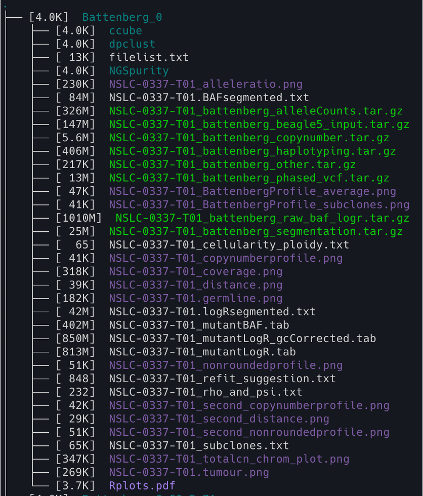
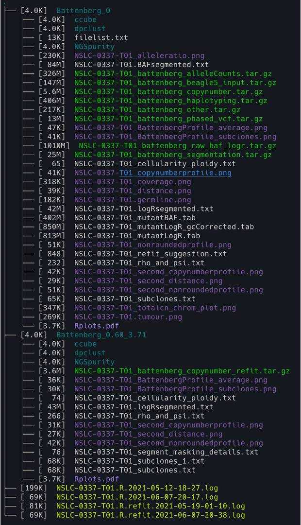
11. You can check the NGSpurity output structure using the following code

tree -lh -C -L 2

• tree: This is the command that generates a tree-like output of the directory structure.
• -lh: This option tells tree to display the file sizes in a “human-readable” format (e.g. using KB, MB, GB suffixes), and to display the file permissions and owner/group information for each file/directory.
• -C: This option tells tree to colorize the output to make it easier to read. Directories will appear in blue and executable files will appear in green.
• -L 2: This option limits the depth of the tree to 2 levels (i.e. only the immediate subdirectories and their contents will be displayed).

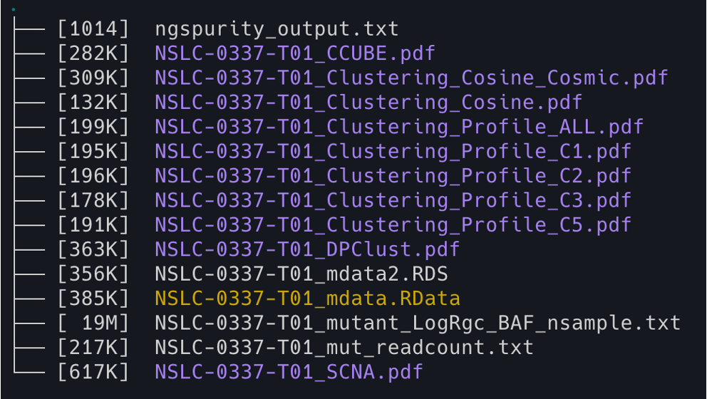
11. You can also check the NGSpurity subfolder using the following code

cd Battenberg_0/NGSpurity && tree -lh -C -L 2

12. Check the major matrix results from NGSpurity (here we use a script ‘verticalize’ to transpose/pivot the output in ‘ngspurity_output.txt’ to a vertical list for better readability).

/data/classes/DCEG_Somatic_Workshop/Practical_session_9/NGSpurity/Library/verticalize ngspurity_output.txt

>>> 2
$1                     Tumor_Barcode : NSLC-0337-T01
$2                               PGA : 0.6135462950203907
$3                     PGA_Subclonal : 0.1488063725107546
$4                         PGA_TETRA : 0
$5                           PGA_LOH : 0.5299956665040626
$6                   PGA_Haploid_LOH : 0.31710993109470564
$7                               MCN : 0.29157255451359027
$8                           MCN_WGD : nWGD
$9                           MCN_CHR : 6
$10                DPClust_Mutations : 5781
$11                     ASCAT_Purity : 0.37
$12                     ASCAT_Ploidy : 1.81182335468724
$13                        BB_Purity : 0.38332
$14                        BB_Ploidy : 1.63516735063955
$15                     CCUBE_Purity : 0.7401220930033857
$16                              GOF : 0.549153609660333
$17                      High_Purity :
$18                   WGD_MP2_Number : 0
$19                    WGD_MP2_Ratio :
$20                   WGD_EVEN_Ratio : 0.08680084182062622
$21                nWGD_CCF_MCluster : 0
$22         nWGD_CCF_MCluster_Detail :
$23         nWGD_Substantial_Segment : 2
$24  nWGD_Substantial_Segment_Detail : chr2:30.68|chr8:17.48
$25                  Super_Cluster_1 : 2
$26                  Super_Cluster_5 : 1
$27                 Super_Cluster_10 : 1
$28             Homozoygous_Deletion : 3
$29            Homozoygous_Deletion2 : Y
$30      Homozoygous_Deletion_Detail : chr13:2:60.24|chr2:1:30.68
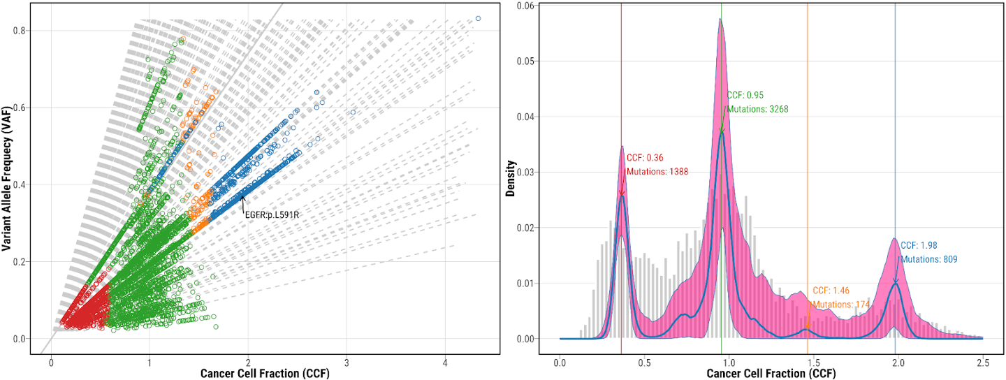
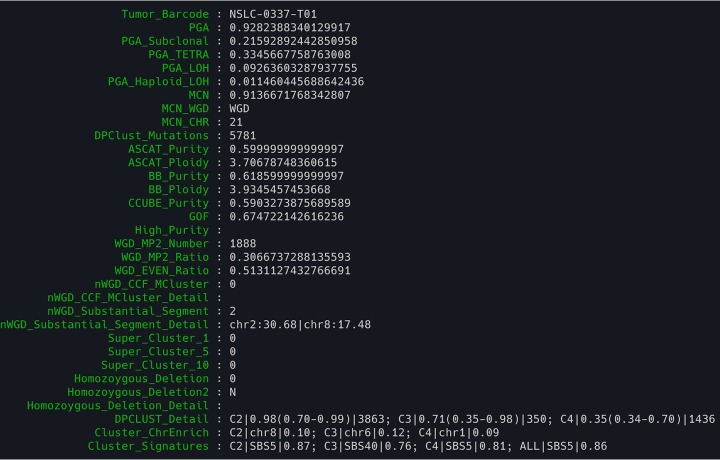
$31                   DPCLUST_Detail : C1|1.98(1.52-2.10)|809; C2|1.46(1.10-1.96)|174; C3|0.95(0.71-1.24)|3268; C5|0.36(0.34-0.75)|1388
$32                Cluster_ChrEnrich : C1|chr2|0.10; C2|chr3|0.15; C3|chr8|0.13; C5|chr3|0.09
$33               Cluster_Signatures : C1|SBS5|0.85; C2|SBS5|0.79; C3|SBS5|0.86; C5|SBS5|0.81; ALL|SBS5|0.86
<<< 2

Example of the annotation for these variables shows below:

1. Tumor_Barcode: NSLC-0001-T01 ((Tumor Barcode, starting with NALC/NSLC/IGC)

2. PGA: 0.9262950347553648 ((Ratio of genomic alteration for SCNA; define as the total length of non-normal state (nMaj!=1 or nMin!=1) of segments devided by total genome size)

3. PGA_Subclonal: 0.10378953433168006 (Same as PGA, but only for subclonal segments; frac<1)

4. PGA_TETRA: 0.128634888054752 (Same as PGA, but limited the segments with nMin=2 and nMaj=2)

5. PGA_LOH: 0.30244654177665375 (Same as PGA, but limited the segments with nMin=0)

6. PGA_Haploid_LOH: 0.025296620914955676 (Same as PGA, but limited the segments with nMin=0 and nMaj=1)

7. MCN: 0.9067952197765827 (percentage of their autosomal genome had an MCN greater than or equal to two; see this paper here)

8. MCN_WGD: WGD (suggested WGD status by MCN; WGD: MCN>0.5; nWGD: MCN<=0.5)

9. MCN_CHR: 21 (How many autosomal chromosomes with MCN>0.5)

10. DPClust_Mutations: 6939 (Number of mutations inlcuded in DPClust or ccube clustering)

11. ASCAT_Purity: 0.16 (Purity estimated by ASCAT)

12. ASCAT_Ploidy: 3.3540227713022 (Ploidy estimated by ASCAT)

13. BB_Purity: 0.15472 (Purity estimated by Battenberg)

14. BB_Ploidy: 3.1786617325949 (Ploidy estimated by Battenberg)

15. CCUBE_Purity: 0.2151671761332141 (Purity estimated by CCUBE)

16. GOF: 0.862975793293232 (Battenberg Godness of Fit)

17. High_Purity: “” (High Purity > 0.95; list the methods estimated as high purity)

18. WGD_MP2_Number: 135 (number of mutations in 2+2 regions have multiplicity 2)

19. WGD_MP2_Ratio: 0.2740740740740741 (Ratio of mutations in 2+2 regions have multiplicity 2; WGD samples >0.95)

20. WGD_EVEN_Ratio: 0.3482940014691765 ratio of segment regions have even major and minor copy number (2+0, 2+2, 4+2, 4+0); WGD smaples < 0.95)

21. nWGD_CCF_MCluster: 0 (Number of mutational clusters with CCF between 0.45 and 0.55 from DPCLUST; nWGD feature)

22. nWGD_CCF_MCluster_Detail: “” (same as nWGD_CCF_MCluster, list the sum all the mutation and ratio)

23. nWGD_Substantial_Segment: 2 (Number of Substantial copy number segments with CCF ~0.5. ‘Substantial’ could be defined as at least 3 segments each >10MB with frac1a between 0.45 and 0.55; nWGD feature)

24. nWGD_Substantial_Segment_Detail: chr5:28.27|chr17:12.48 (same as nWGD_Substantial_Segment, just list the detail for each segment in Mbp)

25. Super_Cluster_1: 0 (Number of superclonal cluster (CCF>1.1) containing more than 1% of mutations)

26. Super_Cluster_5: 0 (Number of superclonal cluster (CCF>1.1) containing more than 5% of mutations)

27. Super_Cluster_10: 0 (Number of superclonal cluster (CCF>1.1) containing more than 10% of mutations)

28. Homozoygous_Deletion: 0 (Number of clonal or subclonal homozygous deletion segments more than 10MB in size)

29. Homozoygous_Deletion2: N (Sum all segments length with clonal or subclonal homozygous deletion; “Y” = length >10MB; “N” = length <=10MB; )

30. Homozoygous_Deletion_Detail: “” (List all clonal or subclonal homozygous deletion segments)

31. DPCLUST_Detail: C2|1.1|6869 (cluster ID | cluster CCF | number of mutations from DPClust; sorted by CCF if muliptle clusters )

32. Cluster_ChrEnrich: C1|chr2|0.10; C2|chr3|0.15; C3|chr8|0.13; C5|chr3|0.09 (list all the enriched chromosome for different clusters)

33. Cluster_Signatures: C1|SBS5|0.85; C2|SBS5|0.79; C3|SBS5|0.86; C5|SBS5|0.81; ALL|SBS5|0.86 (list the most similarity mutational signature for each clusters).

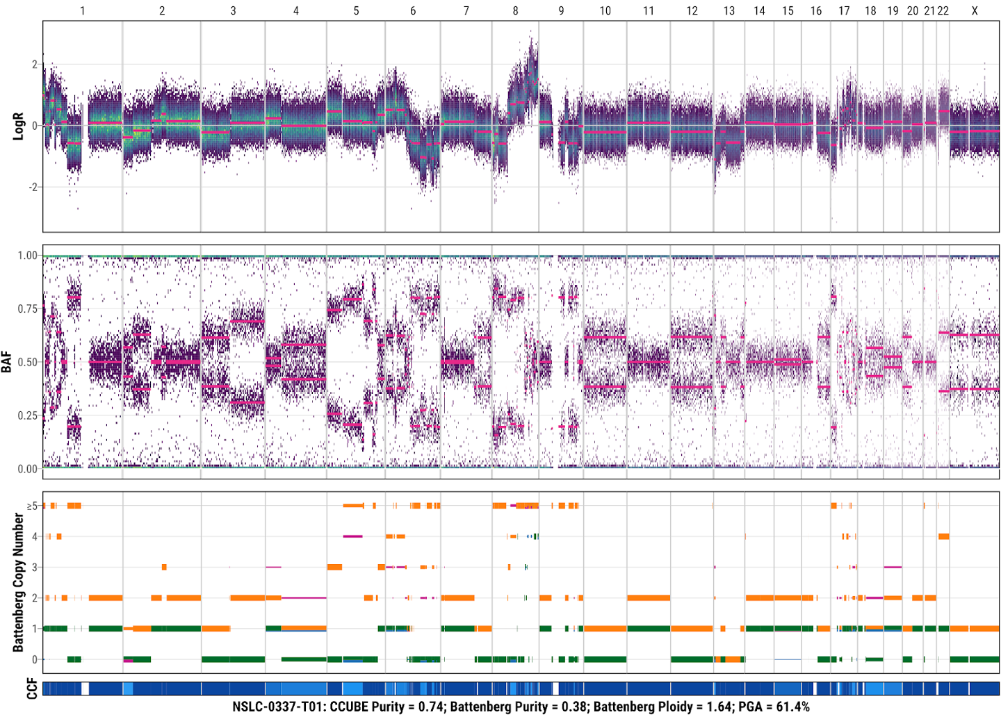
13. Check the SCNA result from the Battenberg

SCNA profiling using Battenberg for tumor NSLC-0037-T01 with the default parameters. Each Battenberg SCNA profile includes LogR, BAF, and absolute copy number (orange: total copy number for major clone; green: minor copy number for major clone; purple: total copy number for additional subclone; blue: minor copy number for additional subclone) and clonality of each segment (dark blue to light blue: ccf from 1 to 0). The tumor sample name, purity estimated by CCUBE, the final purity (Battenberg Purity), final ploidy (Battenberg Ploidy), and percentage of genome altered is shown at the bottom of each Battenberg profile.

14. Check the mutation clustering from DPClust results

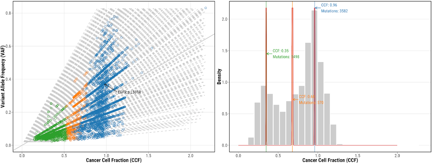
mutation clustering using DPClust for tumor NSLC-0337-T01, which shows both CCF vs VAF scatter plot and CCF distribution. Different colors represent mutations included in different clusters. Potential drive genes are labeled on the clustering plots.

15. Check the mutation clustering from CCUBE results

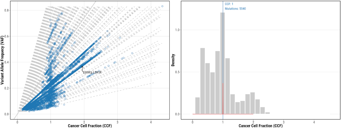
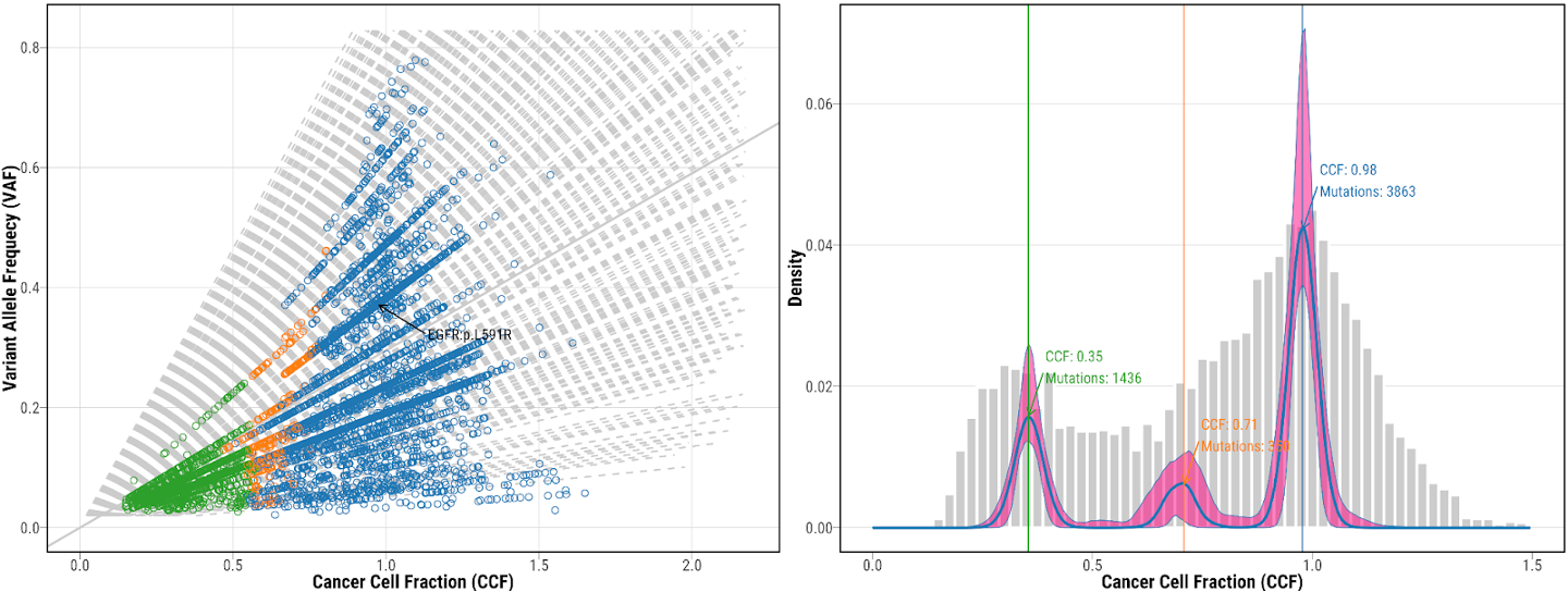
mutation clustering using CCUBE for tumor NSLC-0337-T01, which shows both CCF vs VAF scatter plot and CCF distribution. Different colors represent mutations included in different clusters. Potential drive genes are labeled on the clustering plots.

Refitting Solution for somatic copy number alterations

As shown in cmdfile_refit, We using the following tumor purity and ploidy as the refitting parameters: # Tumor Purity = 0.6, Tumor Ploidy = 3.7

16. check output structures after refitting

17. Check the major matrix results from NGSpurity after refitting

18. Check the SCNA result from the Battenberg after refitting

SCNA profiling using Battenberg for tumor NSLC-0037-T01 with the default parameters. Each Battenberg SCNA profile includes LogR, BAF, and absolute copy number (orange: total copy number for major clone; green: minor copy number for major clone; purple: total copy number for additional subclone; blue: minor copy number for additional subclone) and clonality of each segment (dark blue to light blue: ccf from 1 to 0). The tumor sample name, purity estimated by CCUBE, the final purity (Battenberg Purity), final ploidy (Battenberg Ploidy), and percentage of genome altered is shown at the bottom of each Battenberg profile.

19. Check the mutation clustering from DPClust results after refitting

mutation clustering using DPClust for tumor NSLC-0337-T01, which shows both CCF vs VAF scatter plot and CCF distribution. Different colors represent mutations included in different clusters. Potential drive genes are labeled on the clustering plots.

20. Check the mutation clustering from CCUBE results after refitting

mutation clustering using CCUBE for tumor NSLC-0337-T01, which shows both CCF vs VAF scatter plot and CCF distribution. Different colors represent mutations included in different clusters. Potential drive genes are labeled on the clustering plots.

Palimpsest

From the Palimpsest GitHub:

Cancer genomes are altered by various mutational processes and, like palimpsests, bear the signatures of these successive processes. The Palimpsest R package provides a complete workflow for the characterisation and visualization of mutational signatures, including their evolution along tumor development. The package includes a wide range of functions for extracting single base substitution (SBS), double base substitution (DBS) and indel mutational signatures as well as structural variant (SV) signatures. Palimpsest estimates the probability of each mutation being due to each signature, which allows the clonality of each alteration to be calculated, and the mechanism at the origin of each driver event to be predicted.

In short, Palimpsest is an easy-to-use toolset for the reconstruction of the natural history of tumors using whole exome or whole genome sequencing data.

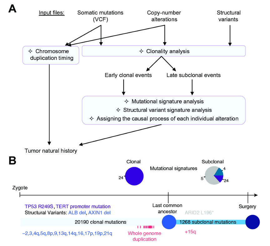
Figure 1. (A) Workflow illustrating a typical analysis with Palimpsest. Taking as input somatic mutations, copy-number alterations (CNAs) and structural variants, the package classifies variants as clonal and subclonal, extracts mutational and structural variant signatures separately in early clonal and late subclonal events, and estimates the probability of each alteration being due to each process. The timing of chromosome duplications is also estimated from the ratio of duplicated/non-duplicated mutations to reconstruct the complete natural history of the tumour. (B) Example of output representing, for one tumour, the number of clonal and subclonal mutations, their distribution per mutation signature, the driver alterations (colored according to the most likely causal mutational process) and CNA timing.

Importing Data and Libraries

We will run the R package Palimpsest using the Palimpsest liver cancer example data and script. Download the scripts here.

The first few steps of this script cover mutational signature extraction and take a while to run. Since we’ve already covered mutational signature extraction in an earlier session we will skip these steps today and begin at step 7 with all signatures extracted.

First we will load the data beginning at line 152:

library(Palimpsest)
library(BSgenome.Hsapiens.UCSC.hg19)
#library(BSgenome.Hsapiens.UCSC.hg38)

setwd("~/Downloads/Palimpsest")
datadir <- "~/Downloads/Palimpsest"

# define parent results directory
resdirparent <- "~/Downloads/Palimpsest/Palimpsest"; if(!file.exists(resdirparent)) dir.create(resdirparent)

load("signaturesextracted.RData")

The minimum requirement for running Palimpsest is a VCF containing mutations, but much of what we demonstrate today will also require purity, SCNA, and ploidy information. Mutational signatures are recommended as they are required to generate the natural history plot above, but they are not required otherwise.

If you do not have mutational signature information, you could begin from step 1 in the script starting with your VCF mutations to extract mutational signatures with the Palimpsest package, though in our experience these extracted signatures are not totally accurate.

We would recommend extracting signatures on your own and feeding those results into Palimpsest for any mutational signature evolution analysis. You can then begin from step 6 where each mutation is assigned a ‘most probable’ origin signature.

Clonality plots and Cancer cell fraction (CCF)

The code in step 7 will produce graphs showing the clonality of mutations:

#-------------------------------------------------------------------------------------------------

# 7] Clonality analysis

#-------------------------------------------------------------------------------------------------

resdir <- file.path(resdir_parent,"Clonality");if(!file.exists(resdir)){dir.create(resdir)}

# Load copy number analysis (CNA) and annotation (annot) data
cna_data = load2object(file.path(datadir,"cna_data.RData"))
annot = load2object(file.path(datadir,"annot_data.RData"))

# Calculate the Cancer Cell Fraction (CCF) of each mutation.
vcf_cna <- cnaCCF_annot(vcf= vcf, annot_data = annot,cna_data = cna_data, CCF_boundary = 0.95)

# Generate graphical representations of clonality analysis
cnaCCF_plots(vcf=vcf_cna,resdir=resdir)

This will generate graphs for each sample in the Palimpsest/Clonality folder.

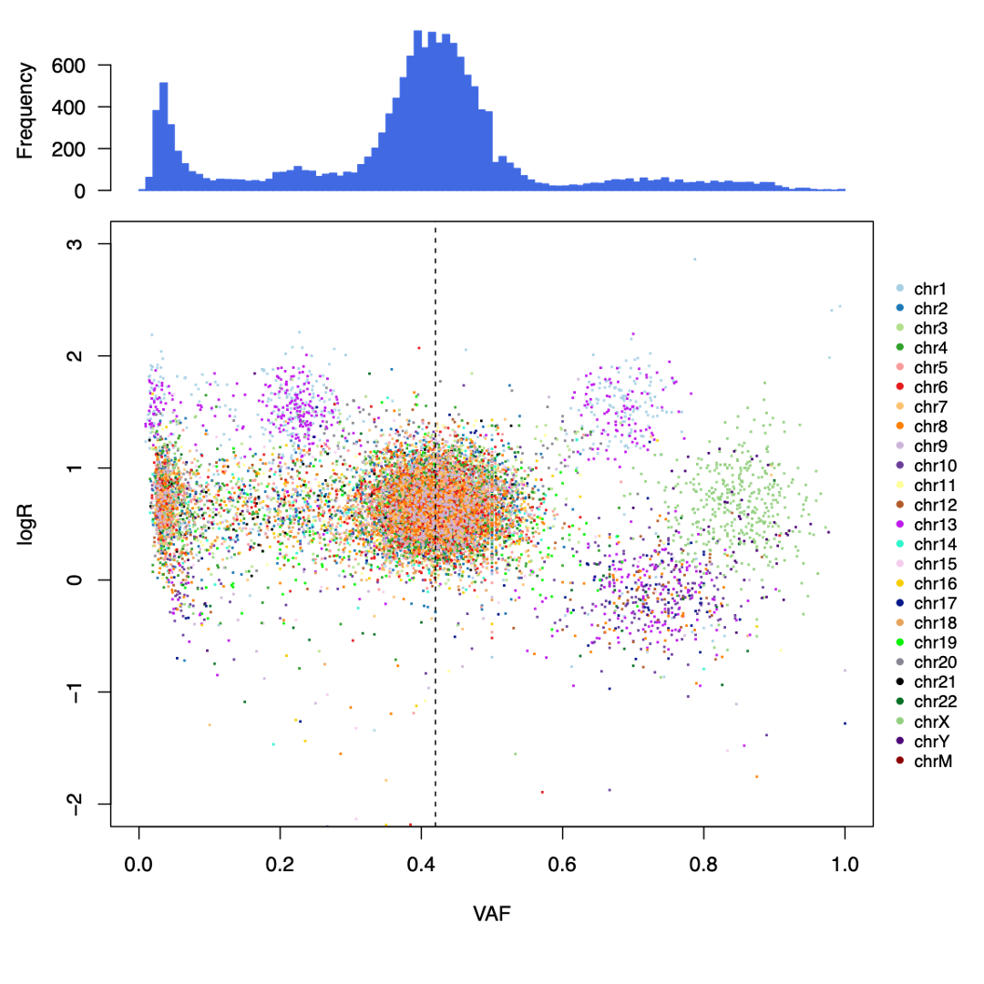
First let us examine the ‘fireworks’ plot of the distribution of VAF on the x plotted against the log2Ratio value as we discussed in session 7 (data for sample CHC2697T). The dashed line is drawn at the expected VAF for heterozygous mutations, taking tumor purity into account, with a histogram of mutations per VAF plotted above.

Somatic deletions will result in mutations with high VAF and low logR (lower-right) and duplications will result in a high logR and more mutations at high and low VAFs, corresponding to mutations on the duplicated and non-duplicated chromosome, respectively (upper-left and -right). Mutations with low VAF (~0.1-0.0) are most likely subclonal, and this is clearly observable as a large peak in the VAF histogram at the top.

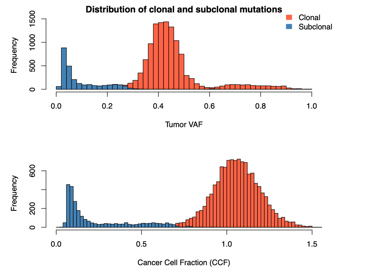
Palimpsest also generates a separate color-coded histogram according to whether mutations are clonal or subclonal.

Temporal evolution of mutational signatures

Next we can use clonality labels for each mutation to separate mutational signatures by clonality.

Note: from here onward we will be using the mutational signatures extracted by the Palimpsest library which we find untrustworthy. This is purely a practical demonstration.

#-------------------------------------------------------------------------------------------------

# 8] Compare mutational signatures between early clonal and late subclonal mutations in each tumour

#-------------------------------------------------------------------------------------------------

resdir <- file.path(resdir_parent,"Signatures_early_vs_late/");if(!file.exists(resdir)){dir.create(resdir)}

# Estimate the contribution of each signature to clonal and subclonal mutations in each tumour
vcf.clonal <- vcf_cna[which(vcf_cna$Clonality=="clonal"),]
SBS_input_clonal <- palimpsest_input(vcf = vcf.clonal,Type = "SBS")
signatures_exp_clonal <- deconvolution_fit(input_matrices = SBS_input_clonal,
                                           input_signatures = SBS_liver_sigs, resdir =  resdir,
                                           save_signatures_exp = F)

vcf.subclonal <- vcf_cna[which(vcf_cna$Clonality=="subclonal"),]
SBS_input_subclonal <- palimpsest_input(vcf = vcf.subclonal,Type = "SBS")
signatures_exp_subclonal <- deconvolution_fit(input_matrices = SBS_input_subclonal,
                                              input_signatures = SBS_liver_sigs, resdir =  resdir,
                                              save_signatures_exp = F)

# Generate per tumour comparisons of clonal and subclonal mutations
palimpsest_DissectSigs(vcf=vcf_cna, signatures_exp_clonal = signatures_exp_clonal,
                       signatures_exp_subclonal = signatures_exp_subclonal,sig_cols = sig_cols,resdir=resdir)

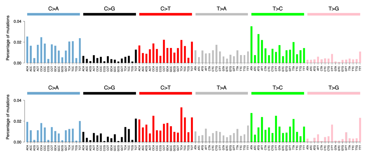
This will produce a graph for each sample in the Palimpsest/Signatures_early_vs_late folder showing the SBS96 category for all clonal (top) and subclonal (bottom) mutations (data for sample CHC2697T).

Using the most probable mutational signature for every mutation (this was calculated beforehand in section 6 of this script before the practical), we can identify when each mutational signature is active in the tumor’s history.

The p-value above the graph (chi-square test) shows whether there are significant differences between clonal and subclonal mutational signatures.

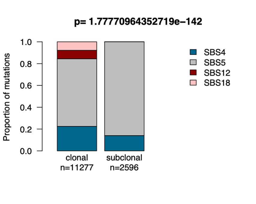
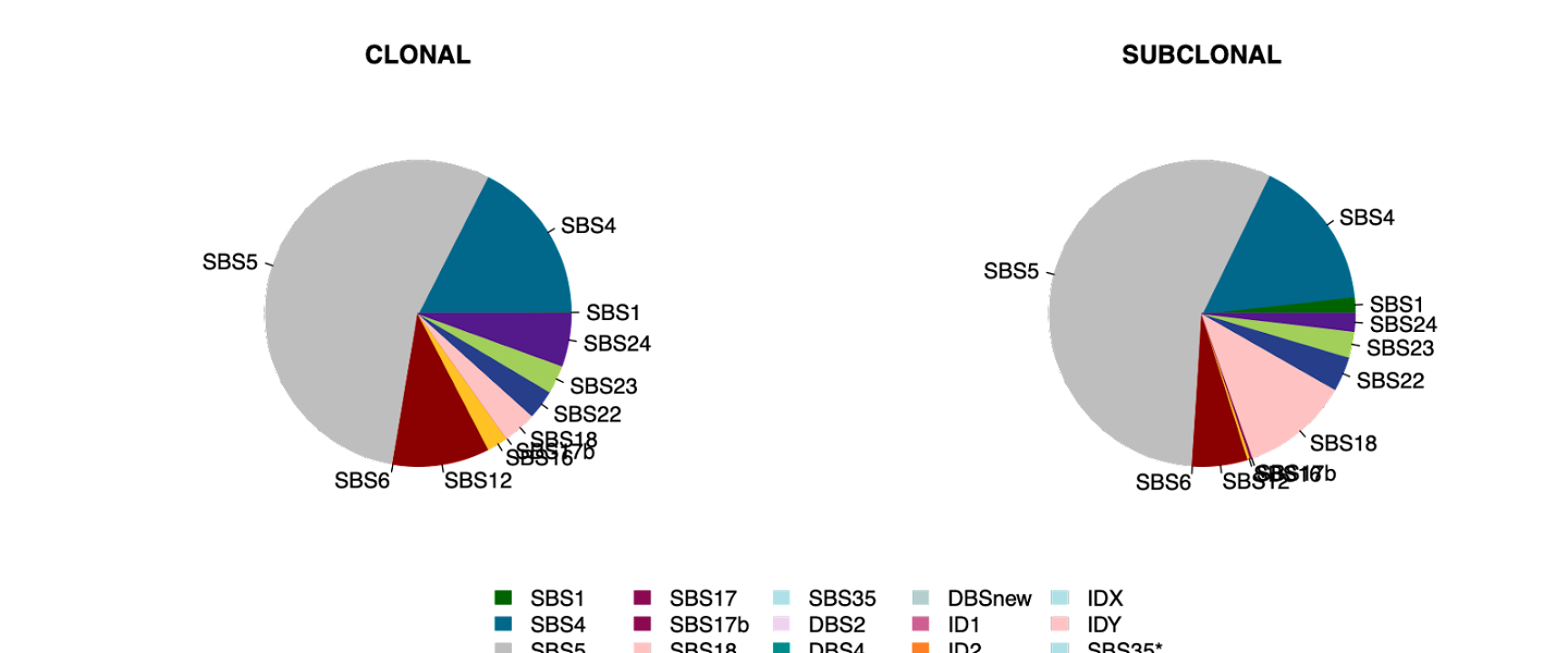
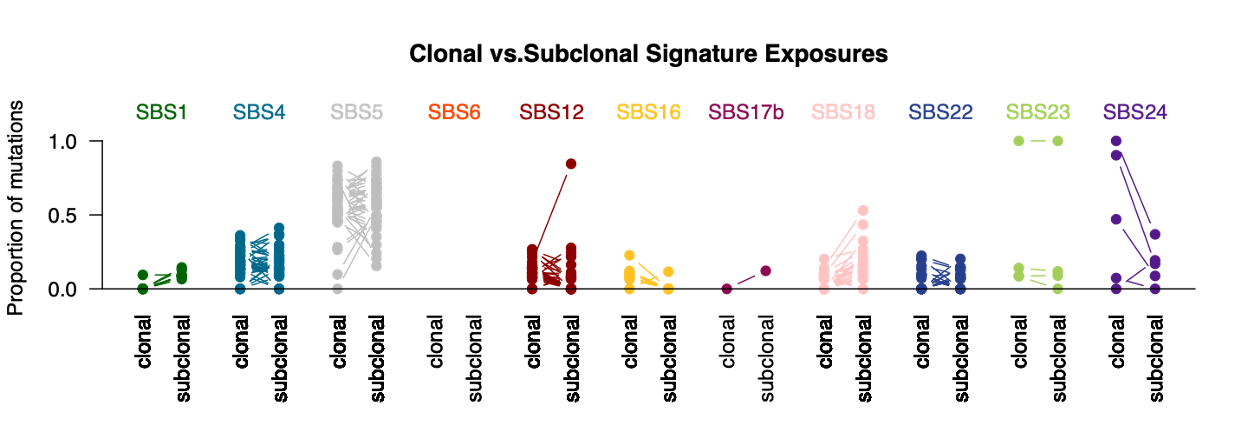
In addition to the prior figures which are calculated on a per-sample basis, we can also visualize clonality of mutational signatures for all samples at once (Clonal_vs_subclonal_series.pdf and Clonal_vs_subclonal_proportions.pdf):

# Generate across the series comparisons of signature assigned to clonal and subclonal mutations
palimpsest_clonalitySigsCompare(clonsig = signatures_exp_clonal$sig_nums,
                                subsig = signatures_exp_subclonal$sig_nums, msigcol = sig_cols, resdir = resdir)

dev.off()

Here we can see signature SBS18 is more often subclonal (later progression mutations) whereas SBS24 predominantly causes early, clonal mutations.

Copy number alterations

Next we can identify copy number alterations and time these changes.

#-------------------------------------------------------------------------------------------------

# 9] Timing Chromosomal Gains

#-------------------------------------------------------------------------------------------------

resdir <- file.path(resdir_parent,"ChromosomeDups_timing/");if(!file.exists(resdir)){dir.create(resdir)}

# Annotate vcf with chromomal gain timings
chrom_dup_time <- chrTime_annot(vcf=vcf_cna,cna_data = cna_data,cyto=cytoband_hg19)
vcf_cna <- chrom_dup_time$vcf;point.mut.time <- chrom_dup_time$point.mut.time;cna_data <- chrom_dup_time$cna_data

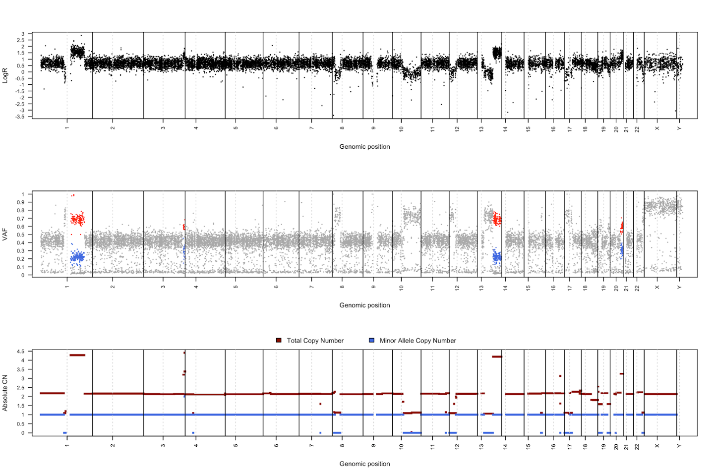
This will generate a figure for each sample in folder Palimpsest/ChromosomeDups_timing combining logR and VAF information to calculate copy number as discussed in session 7. The final panel gives a summary of the estimated copy number and minor allele copy number across the genome.

By examining the ratio of variants with a high VAF (red) vs low VAF (blue), we can infer how many mutations were acquired at the time of the chromosomal duplication:

• a very even distribution of variants between high and low VAF indicates that most mutations were present at the time of chromosome duplication, i.e. a late duplication
• an early duplication will result in very few duplicated mutations, which will be low VAF due to the duplication

# Visualising timing plots

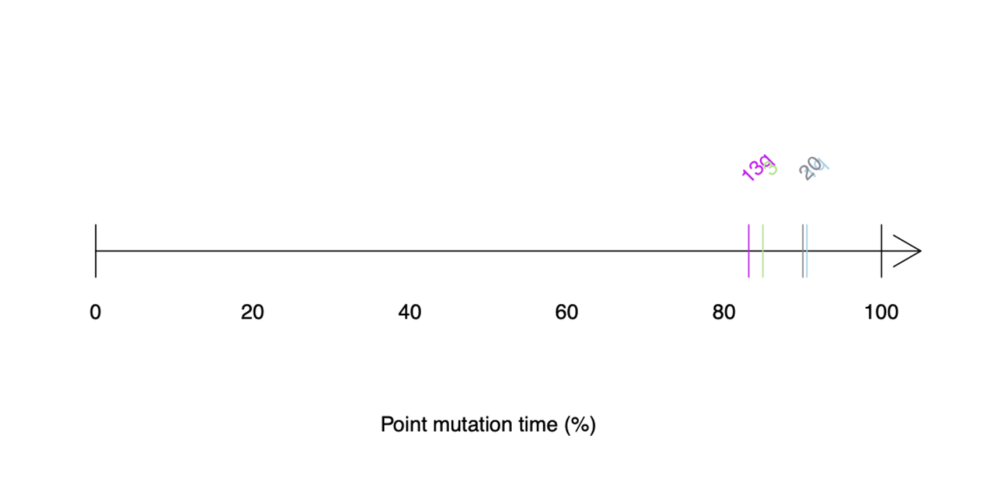
chrTime_plot(vcf = vcf_cna, point.mut.time = point.mut.time, resdir = resdir,cyto = cytoband_hg19)

Deletions cannot be estimated because the VAF of all mutations will be simply homozygous regardless of timing.

Natural history of tumors

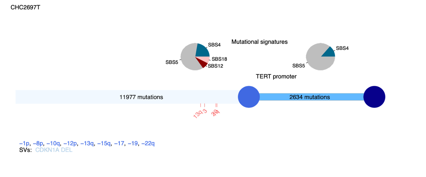
Finally we can combine all of the previous results to create a combined plot which clearly outlines the evolutionary history for each tumor.

#-------------------------------------------------------------------------------------------------

# 11] Visualise the natural history of tumour samples:

#-------------------------------------------------------------------------------------------------

resdir <- file.path(resdir_parent,"Natural_history/");if(!file.exists(resdir)){dir.create(resdir)}

palimpsest_plotTumorHistories(vcf = vcf_cna, sv.vcf = SV.vcf,cna_data =  cna_data,
                              point.mut.time = point.mut.time,
                              clonsig = signatures_exp_clonal$sig_props,
                              subsig = signatures_exp_subclonal$sig_props,
                              msigcol = sig_cols, msigcol.sv = SV_cols, resdir = resdir)

This will generate figures for each sample in the folder Palimpsest/Natural_history:

Events before the first blue circle are clonal events, those between the two circles are subclonal.