This practical section will focus first on connecting to a remote cluster as well as using the linux command line. Then we will practice working with some common bioinformatics file formats.
Speakers: Wei Zhao
Setup ssh connection
First, to use the computing clusters we need to establish an ssh connection between your computer and the cluster.
The steps to do this will differ depending on whether you’re using MacOS or Windows:
MacOS
- Open the Terminal app, like so:
- “Finder -> Applications -> Utilities -> Terminal”
- enter the following command:
ssh USERNAME@biowulf.nih.gov, replacing ‘USERNAME’ with your own username.
Windows
-
Download PuTTY. The version ‘putty.exe’ is a standalone package that does not require installation.
-
Launch PuTTY. Under “Host Name (or IP address), type:
USERNAME@biowulf.nih.gov, replacing ‘USERNAME’ with your own username, and click “Open”

- At the prompt, enter the account password. Please note that the password will not show on the screen, and 5 failed login attempts since the last successful login are allowed.
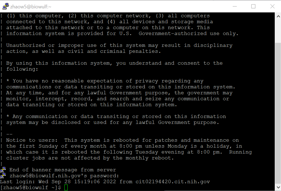
At this point you should be connected to the NIH Biowulf cluster, and your screen should look something like this:
Request an interactive session
You’re now logged into the login nodes that are shared by everyone who uses Biowulf. It is important that you do NOT run intensive computing jobs on the login nodes to make them overburdened. If you do, other users will be temporarily unable to use Biowulf. You should instead request an interactive session, then you will be assigned to the compute nodes.
To do this, type this command:
sinteractive --mem=4g --cpus-per-task=2 --time=4:00:00
and hit enter.
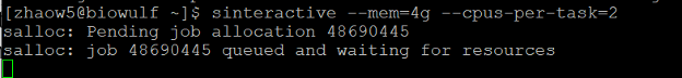
You will see this screen when your request has been submitted and is waiting for computing resources:
When you are allocated to a compute node you should see USERNAME@cn####, like this:

When you want to close the interactive session use the command exit, and you will return to the login nodes.
Locally mounting HPC System Directories
We will need to mount your personal /data drive to access files on Biowulf from your local computer at the end of this session. See the instructions here for mounting your data directory: (https://hpc.nih.gov/docs/hpcdrive.html).
Basic Bash/Linux commands
Now let’s practice some basic linux commands:
1. First, let’s check what directory we’re working in on the command line. Simply type:
pwd
and hit enter. This should output /home/[your username].
2. Since Biowulf home directories are relatively small we are going to be working in the /data/ directory, so let’s make a folder there with the mkdir command:
mkdir /data/[your username]/session1
To verify that your folder was created successfully, enter the following: ls /data/[your username]. This should list all contents of your /data/ directory, and among those contents should be the ‘session1’ folder.
3. Let’s move ourselves to that directory to begin working:
cd /data/[your username]/session1
Verify that you are in the right folder with the pwd command.
4. Let’s copy some files to practice with. We deposited two copies of our sample data in Biowulf and Github, respectively. You can follow either 4a or 4b to copy the data to your home directory.
4a. Copy the data from the shared folder in Biowulf. Before we do that, let’s look at the contents of the course folder like so:
ls -lh /data/classes/DCEG_Somatic_Workshop/Practical_session_1
Now let’s copy that data over to our current directory:
cp -r /data/classes/DCEG_Somatic_Workshop/Practical_session_1/* .
The option -r means copy directories recursively (i.e. including all the contents in sub-directories). If we omit this option, all the folders in this directory will be skipped.
The last two characters in the code above are special characters with specific meanings. The * in the code above is called a ‘wildcard’ and can be interpreted as ‘anything’. In words, we’re instructing the computer to copy all files in /data/classes/DCEG_Somatic_Workshop/ matching the pattern ‘anything’, or in other words all files.
The . in the code means ‘the current working directory’, and is where we’re copying the files to.
4b. Alternatively, you can download the data from GitHub.
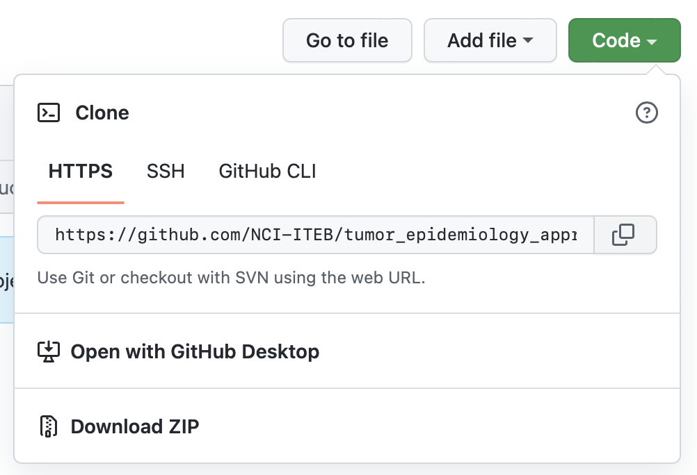
Let’s first look up the link from GitHub. Open the course resources in web browser: https://github.com/NCI-ITEB/tumor_epidemiology_approaches_materials
Click the green button ‘code’. Click the button next to the https link to copy the link.
With the link now copied to your clipboard, return to the Biowulf terminal and enter git clone followed by the link you’ve copied:
git clone https://github.com/NCI-ITEB/tumor_epidemiology_approaches_materials.git
5. Now we can switch to the directory of the sample input data.
cd sample_input_data
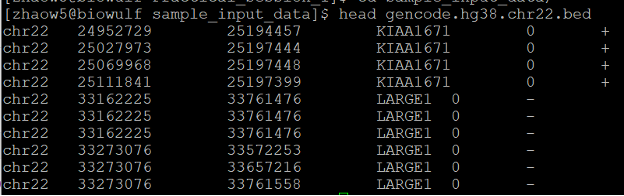
There is a BED file with transcript coordinates in chromosome 22 (gencode.hg38.chr22.bed). Let’s check the first few lines of this file:
head gencode.hg38.chr22.bed
By default, head will give you the first ten lines of a file to examine. If you want to see more, you can use the option -n, or examine the file manually with the more command.
6. Finally let’s try sorting this BED file (gencode.hg38.chr22.bed) by genomic coordinates. Note that many commands/applications will require the input files (in BAM or BED formats) to be sorted by genomic cooridinates.
But before we do that let’s first check the manual on the sort command:
man sort
Use the arrow keys or your scroll wheel to read, and take note of the options -k and -r. To exit the manual enter q.
Then we can sort the file with this command:
sort -k1,1 -k2,2n gencode.hg38.chr22.bed >gencode.hg38.chr22.sorted.bed
-k1,1 -k2,2n: sort first by the first field, then by the second field numerically. The sorting isn’t saved automatically, so as before we use the > to redirect the output to a new file.
Working with FASTQ files
7. Before we can work with our fastq files we need to decompress them using the decompression command tar:
tar -xzvf Sample1.tar.gz
The -xz and -f options tell tar that we want to decompress our files and what file to extract from, respectively. The -v option is to print filenames as they’re decompressed.
8. Let’s preview our files. We can do it in two ways:
head Sample1_1.fq
We have used the head command before. This will return the first ten lines of the file by default.
Alternatively, we can use:
more Sample1_1.fq
Use ‘enter’ or ‘space’ to scroll down, ‘b’ to scroll back, and ‘/’ to search. To quit, either reach the end of the file or type q.
We have another compressed format for the same file (files with extension .fastq.gz). We can check the contents of these files directly without creating a plain text file, using this command:
zless Sample1_1.fastq.gz
Same to the command more, use ‘space’ to scroll down, and type q to exit.
To check the number of paired-end reads, use the following commands:
echo $(zcat Sample1_1.fastq.gz | wc -l)/4 | bc
echo $(zcat Sample1_2.fastq.gz | wc -l)/4 | bc
You should see ‘300,000’ for both commands.
To briefly explain these commands:
zcat Sample1_1.fastq.gz | wc -l: print the decompressed contents of the gzipped (‘.gz’) reads file using ‘zcat’, then count the number of lines by feeding (or piping, the ‘|’ symbol) the output directly to ‘wc -l’echo $(...)/4 | bc: setup a division by 4 of the line count value from thewc -lcommand usingecho(recall that each sequence in the fastq is composed of four lines). This mathematical expression is only evaluated after using the commandbc.
9. Let’s subset our fastq file to a smaller collection of reads with the seqtk library. First load seqtk:
module load seqtk
10. then use the ‘subseq’ tool to extract the reads specified in the ‘name.lst’ file:
seqtk subseq Sample1_1.fq name.lst >out.fq
‘name.lst’ is a list of identifiers of reads.
head name.lst
Check the output file ‘out.fq’ with the head and/or more command.
Working with BAM files
11. We’re going to be working with BAM files from 1000 genomes. The example data was downloaded from the 1000 Genomes Project.

We used the following command to download the example in this session:
samtools view http://s3.amazonaws.com/1000genomes/1000G_2504_high_coverage/data/ERR3240193/HG00118.final.cram chr22:38952741-38992778
And the CRAM file could be converted to BAM using this command:
samtools view -h -b -@ 10 -T Homo_sapiens_assembly38.fasta -o HG00118__chr22@38952741@38992778.bam HG00118__chr22@38952741@38992778.cram
12. Now we rename the BAM file in our input data folder to reads.bam.
mv HG00118__chr22@38952741@38992778.bam reads.bam
Examine file format
13. Let’s look at the header of this BAM file. Try listing all the versions of samtools available on Biowulf:
module spider samtools
Some modules will have different parameters in different versions. By default, usually it will load the latest version of the module. For our purposes any recent version will suffice, so enter module load samtools to load the default version of samtools. Then to view the BAM header, enter:
samtools view -H reads.bam | more
The view mode of samtools is a tool to print sections of a BAM/SAM/CRAM file, and the -H option instructs samtools to print only the header. In this example we then feed the samtools output directly to the more command via the linux ‘pipe’ (the | symbol) so it’s easier to read and browse.
Note that we’ve been using a BAM file which is in binary format, but the output is in readable text. Samtools has converted the output from BAM to SAM automatically.
If we want to extract specific fields in the header, we could use the grep command. For example, this command would extract the lines for read groups in the header.
samtools view -H reads.bam|grep "^@RG"
The ^ symbol will match all lines starting with a specific pattern. In this example, it matches all lines starting with “@RG”. Purely for your interest, these are the read group definition lines.
14. Now let’s view the first 20 lines of the aligned reads in the body section. The command will be very similar, but without the -H option samtools will ignore the header:
samtools view reads.bam|head -20
As before, we use the pipe to feed the output into the head -20 command so we can see just the first 20 lines.
Extract, sort, index reads
15. Let’s isolate only unmapped reads, and reads with unmapped mates:
samtools view -b -f4 reads.bam >unmapped.bam
samtools view -b -f8 reads.bam >mate_unmapped.bam
The -b flag tells samtools to output in the compressed BAM format rather than SAM, and is very important when working with large alignment files. The -f flag requires all output reads to have the specified alignment flags, in this case flag ‘4’ and flag ‘8’. These correspond to ‘read unmapped’ and ‘mate unmapped’, respectively.
A full list of SAM flags can be found at: https://broadinstitute.github.io/picard/explain-flags.html
16. Sort the original file by genomic coordinates and output into file reads_sorted.bam:
samtools sort -o reads_sorted.bam reads.bam
Note that in the previous command we used > to save a new file whereas in this case we’ve used -o [file name] to accomplish the same.
17. Let’s now index the sorted file. Indexing allows for more efficient lookup of reads and is required to run many bioinformatics algorithms:
samtools index reads_sorted.bam
This should create a new index file reads_sorted.bam.bai.
18. Take a look at some of the alignment statistics using:
samtools flagstat reads_sorted.bam
19. Find all reads mapping to chr22:38,700,000-39,300,000 and save to file chr22.bam:
samtools view -h -b reads_sorted.bam chr22:38,700,000-39,300,000 > chr22.bam
The -h option will retain the original header in our output file.
Working with BED files
20. Let’s convert our chr2 BAM alignment file to BED format. First load bedtools and then use the ‘bamtobed’ mode:
module load bedtools
bedtools bamtobed -i chr22.bam > reads.bed
21. For each gene that overlaps with alignments, report the base-pair overlap between the sequence alignment and genes. Here we can use the ‘reads.bed’ file to extract all the regions with alignments.
bedtools intersect -a reads.bed -b gencode.hg38.chr22.sorted.bed >intersect_overlap.bed
-a and -b specify our two BED file inputs.
22. For each gene that overlaps with alignments, report the full-length of the original gene. Report each gene with more than one hit only once.
bedtools intersect -a gencode.hg38.chr22.sorted.bed -b reads.bed -wa -u >intersect_full_length_genes.bed
Compare to 21, note that we have a -wa option in 22. See the diagram below for the specifics on bedtools intersect.
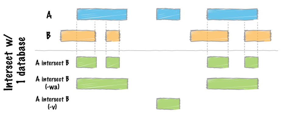
With the option -u, each read with more than one hit will be reported only once.
23. Report regions in genes that have no overlap with alignments (specified with -v):
bedtools intersect -a gencode.hg38.chr22.sorted.bed -b reads.bed -v >intersect_no_overlap.bed
24. For a more advanced query, we can do the following: report all reads within 2000bp upstream or 1000bp downstream of genes.
bedtools window -a reads.bed -b gencode.hg38.chr22.sorted.bed -l 2000 -r 1000 -u > intersect_reads_window.bed
The options -l and -r (‘left’ and ‘right’) define the base pair window upstream and downstream of the overlapping regions, respectively.
Visualizing on UCSC
25. We’re going to visualize these reads on UCSC, and to do so we need to add some header lines to our BED file. Run the following series of commands (red text only):
- Configure browser:
printf "browser position chr22:38,700,000-39,300,000\nbrowser hide all\n" > custom_UCSC_track.bed
- Add the track for overlapping regions:
(printf "track name=\"overlap regions\" description=\"example for bedtools A intersect B\" visibility=1 color=0,0,255 useScore=1\n#chrom\tchromStart\tchromEnd\tname\tscore\tstrand\n" && cat intersect_overlap.bed) >> custom_UCSC_track.bed
- Add the track for full length of genes:
(printf "track name=\"original genes\" description=\"example for bedtools A intersect B -wa\" visibility=3 color=255,0,0 useScore=1\n#chrom\tchromStart\tchromEnd\tname\tscore\tstrand\n" && cat intersect_full_length_genes.bed) >> custom_UCSC_track.bed
The printf and cat commands simply print some text which we then save to a file using >. Take a look at this header we’ve just created using head custom_UCSC_track.bed
.
Note one very important detail in the previous commands: >> will append text to the end of an existing file while > will overwrite existing files. When working with files of your own, be very careful of this difference or you could accidentally lose data!
26. Let’s now visualize using the UCSC genome browser. Go to https://genome.ucsc.edu/. Under the “Genomes” tab, select “Human GRCh38/hg38” and then click the ‘add custom tracks’ button on the bottom of the genome browser.
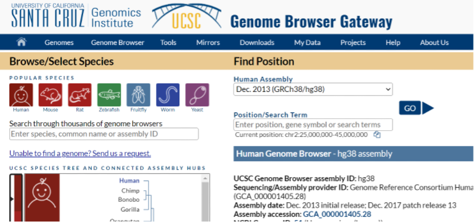
Next, upload the BED file via the “Choose File” button


and finally hit “go”. An APOBEC3B homozygous deletion is highlighted below.
