Session 9: Tumor Evolution

Multi-Region Sequencing Analysis

Now we will practice using the REVOLVER R package (https://caravagnalab.github.io/revolver/index.html) to analyze clonal and subclonal evolution from a multi-region tumor studies. We will use the example data from this study on colorectal adenocarcinoma: https://pubmed.ncbi.nlm.nih.gov/30177804/.

First, if you have not already downloaded the necessary packages, download REVOLVER like so:

if(!require(devtools)){
install.packages("devtools")
}
devtools::install_github("https://github.com/caravagnalab/revolver")

Next, load the necessary libraries:

library(revolver)
library(evoverse.datasets)

Now we must load the dataset, like so:

data(CROSS_CRC_ADENOCARCINOMA_NATECOEVO_2018, package = 'evoverse.datasets')
print(CROSS_CRC_ADENOCARCINOMA_NATECOEVO_2018)

The required columns for input are as follows:

The CCF column is a string showing the CCF of each mutation in every region, like so: ‘R1:0.7;R2:1;…’ etc. for each region.

The first thing to do is to transform this data into a ‘revolver cohort’ object with the revolver_cohort function:

CROSS_CRC_ADENOCARCINOMA_REVOLVER = revolver_cohort(  
CROSS_CRC_ADENOCARCINOMA_NATECOEVO_2018,   
MIN.CLUSTER.SIZE = 0,
annotation = "Colorectal adenocarcinomas (Cross et al, PMID 30177804)")

Once that is complete we need to remove drivers which are present in only one sample. REVOLVER seeks to characterize repeated evolutionary patterns in cancer development and also leverages evolutionary patterns across samples to order mutations which would otherwise be impossible to order, such as ordering of clonal mutations in a sample. For both of these reasons, single driver events are not useful.

## Collect names of drivers occuring only once, then remove from the cohort
non_recurrent = Stats_drivers(CROSS_CRC_ADENOCARCINOMA_REVOLVER) %>%
  filter(N_tot == 1) %>%
  pull(variantID)

CROSS_CRC_ADENOCARCINOMA_REVOLVER = remove_drivers(CROSS_CRC_ADENOCARCINOMA_REVOLVER, non_recurrent)

Next, we will construct mutation trees for each sample and run hierarchical clustering to group sample into clusters of similar evolutionary history.

## Build mutation trees
CROSS_CRC_ADENOCARCINOMA_REVOLVER = compute_mutation_trees(CROSS_CRC_ADENOCARCINOMA_REVOLVER)

CROSS_CRC_ADENOCARCINOMA_REVOLVER = revolver_fit( CROSS_CRC_ADENOCARCINOMA_REVOLVER,
  parallel = F,
  n = 3,
  initial.solution = NA)

## Run hierarchical clustering
CROSS_CRC_ADENOCARCINOMA_REVOLVER = revolver_cluster(CROSS_CRC_ADENOCARCINOMA_REVOLVER,
split.method = 'cutreeHybrid',
min.group.size = 3)

Now we can generate plots for our samples. First we will plot the clustered samples based on their evolutionary trajectories:

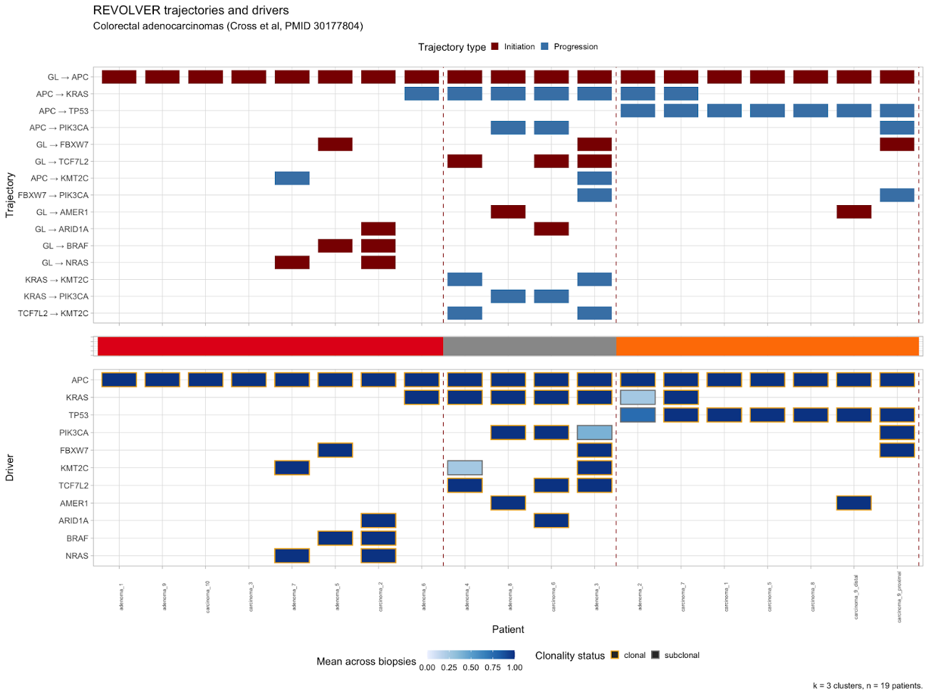
plot_clusters(CROSS_CRC_ADENOCARCINOMA_REVOLVER, cutoff_trajectories = 1, cutoff_drivers = 0)

Here we can see in the third cluster, samples all share APC->TP53 as a progression. The middle cluster has many samples with APC->KRAS along with other initiation events and progressions from KRAS->KMT2C or ->PIK3CA progression. The first cluster has APC initiation but very few progression events. Note that in this and all following graphs, ‘GL’ means germline or the ‘normal’ ancestor of the cancer.

To see these clusters at a higher level:

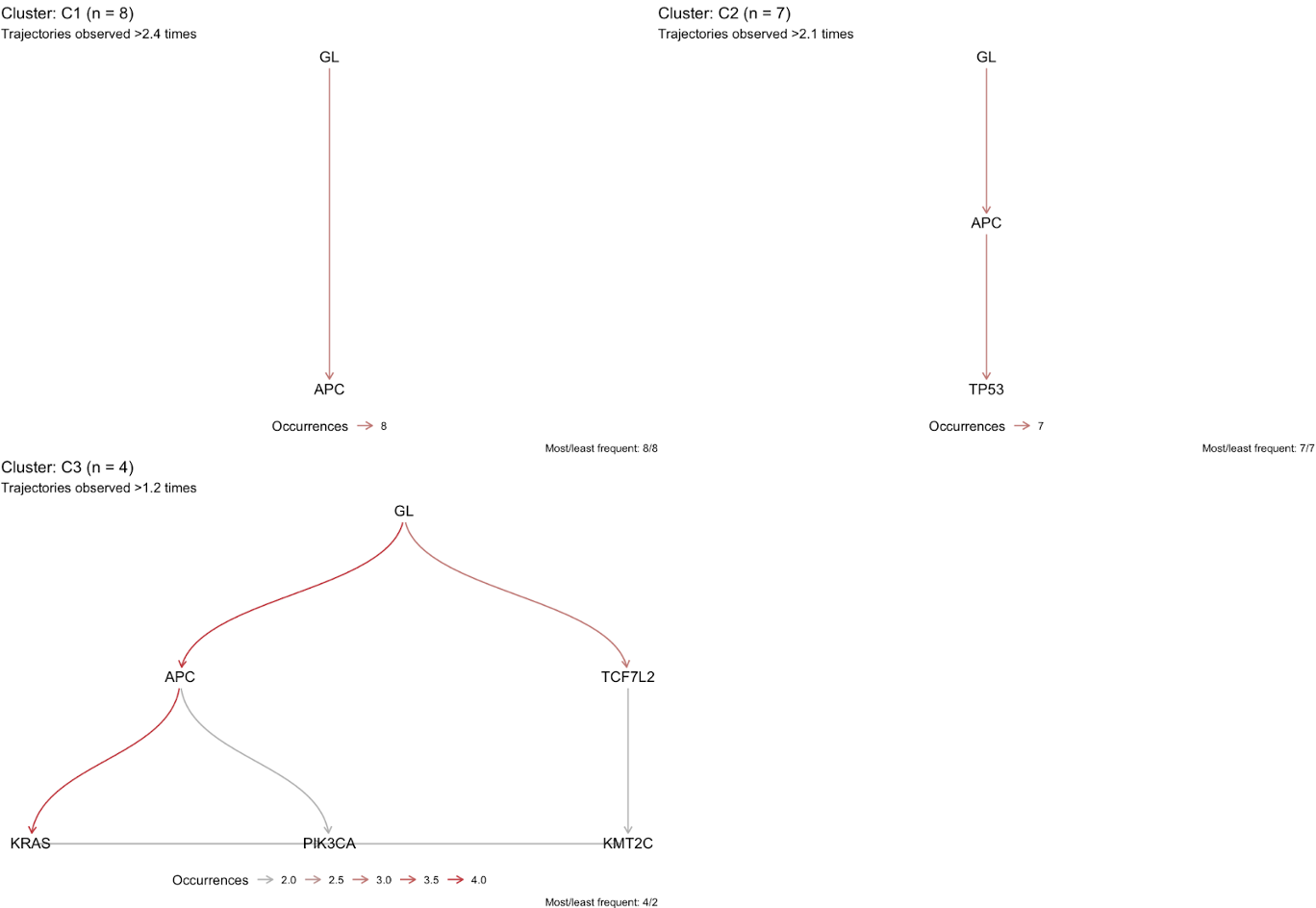
plot_trajectories_per_cluster(CROSS_CRC_ADENOCARCINOMA_REVOLVER, min_counts = .3)

This will give a clear picture of what features characterize each cluster most strongly (as determined by the minimum proportion of samples in that cluster via min_counts).

Lastly, we can view the overall mutation pattern in our cohort with a ‘drivers’ graph, like so:

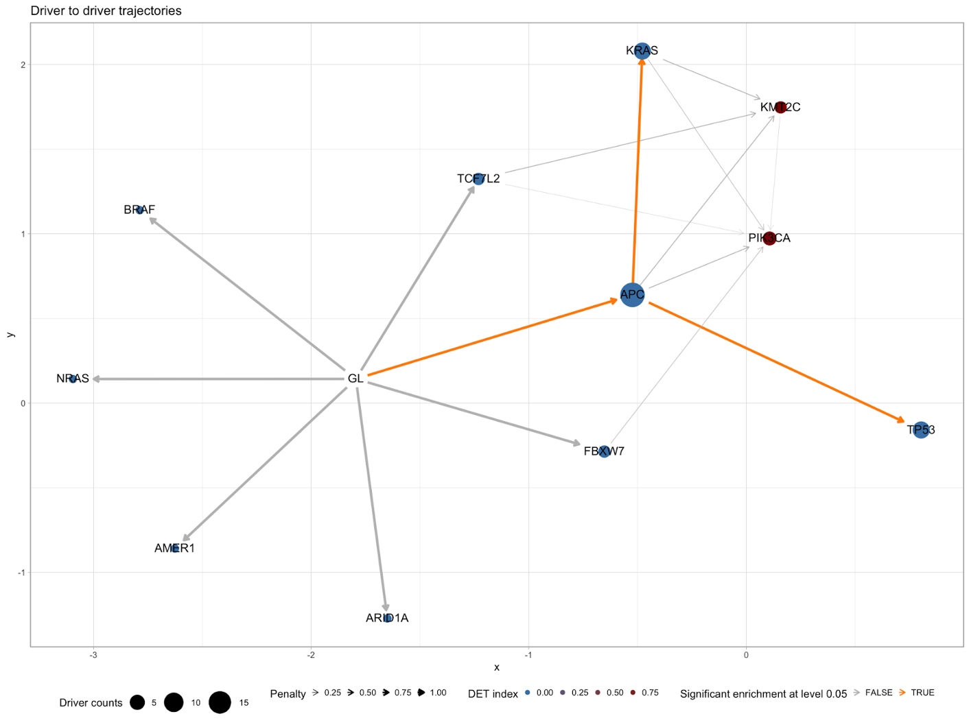
plot_drivers_graph(CROSS_CRC_ADENOCARCINOMA_REVOLVER)

Here we can see a very clear flowchart beginning from ‘GL’/germline and showing the different initiation and progression paths.