Session 3: DNA Sequencing Strategies and Quality Control

Presenters: John McElderry, Phuc Hoang

Before we begin, please login to Biowulf and request an interactive session:

For a reminder on how to log-in to Biowulf, we refer you to this Biowulf HPC guide. In short:

• (Windows) use PuTTy
• (Mac) enter ssh USERNAME@biowulf.nih.gov to your terminal, then enter your password

Request an interactive session with: sinteractive

The purpose of this practical session is for you to gain hands-on experience performing quality control (QC) on sequencing data.

Today’s tasks will include generating and examining FastQC reports of fastq data, followed by adapter trimming. We will then perform some alignment-level quality control on pre-generated alignment files using a variety of tools, and collect these various QC reports into one interactive report file using MultiQC.

Finally, we will highlight some QC metrics that are particularly important for targeted sequencing, whole-exome sequencing (WES), or whole-genome sequencing (WGS).

Running the QC script

We will use three WES samples sequenced with the same exome capture kit (SeqCap EZ Exome + UTR V3) for the bulk of this practical:

• One sample derived from frozen tumor tissue (Fresh_Frozen.bam)
• A second tumor derived from a Formalin-Fixed Paraffin-Embedded (FFPE) sample (FFPE_Tumor.bam)
• A third sample derived from normal blood (LC_LC_IGC-11-1100_A.bam), which we will use for only a few demonstrations

Because our tasks for today will require nearly 20 mins computation running time, we will submit our QC script to Biowulf at the very beginning of this section so that it has time to complete.

1. After logging in, move to your personal data folder to create a folder for the practical session and move to that folder:

cd /data/$USER/
mkdir practical_session_3
cd practical_session_3

2. Copy over the script that will run today’s analyses, like so:

cp /data/classes/DCEG_Somatic_Workshop/Practical_session_3/practical_3_script.sh .

3. Once that’s copied we’ll go ahead and submit this script to Biowulf and request 8 cpus and 8GB of memory to speed up the analysis:

sbatch --cpus-per-task 8 --mem 8g practical_3_script.sh

If you’ve successfully submitted a job, Biowulf should return an eight-digit number corresponding to the ID of your job, like so:

4. Once the job is submitted you can check the status of your job by simply typing and entering sjobs.

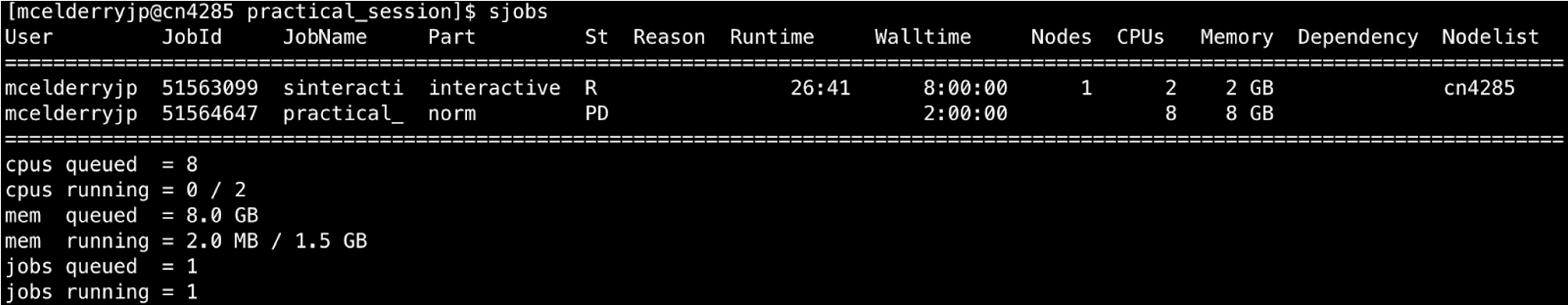
This will give a report of jobs you have queued or running and their status. Alternatively for a graphical display of job status with more advanced statistics you can check the Biowulf User Dashboard.

You should also see a file slurm-########.out in your directory once your job begins running (check with ls). This is an output file containing the text that would normally be written to the command line if you were to run these programs interactively (i.e. not via Biowulf job submission). It is a log for your script, and if your output is not what you expected or a job fails you would want to check this file to get details for troubleshooting.

5. Let’s now examine the script. To do this we will use the program vi, which as we mentioned in lecture 1 is a text editor for the command line:

vi practical_3_script.sh

practical_3_script.sh:

#!/usr/bin/env bash

## Set path to where class files are being stored
PATH_TO_PRACTICE3=/data/classes/DCEG_Somatic_Workshop/Practical_session_3
mkdir practical_3
OUTDIR=practical_3
CPUS_PER_COMMAND=3

## Load modules for running QC analysis
module load fastqc
module load trimgalore
module load samtools
module load R
module load picard
module load multiqc
module load mosdepth

mkdir $OUTDIR/fastqc_out $OUTDIR/trimgalore_out
## Run fastqc on all fastq files
fastqc -t $CPUS_PER_COMMAND -o $OUTDIR/fastqc_out \
$PATH_TO_PRACTICE3/sample_data/germline_EAGLE_WES/LC_LC_IGC-11-1100_A.bam \
$PATH_TO_PRACTICE3/sample_data/Fresh_Frozen/Fresh_Frozen.bam \
$PATH_TO_PRACTICE3/sample_data/FFPE/FFPE_Tumor.bam &

## Perform adapter/low quality base trimming on smaller fastq samples
trim_galore -j $CPUS_PER_COMMAND --fastqc --paired --gzip --stringency 3 \
-o $OUTDIR/trimgalore_out --basename trimmed-LC_LC_IGC-11-1100_A \
$PATH_TO_PRACTICE3/sample_data/germline_EAGLE_WES/LC_LC_IGC-11-1100_A.bam.fq1.gz \
$PATH_TO_PRACTICE3/sample_data/germline_EAGLE_WES/LC_LC_IGC-11-1100_A.bam.fq2.gz &
wait

mkdir $OUTDIR/samtools_out $OUTDIR/picard_inserts_out
## Calculate alignment flag statistics using Samtools
samtools flagstat -@ $CPUS_PER_COMMAND \
$PATH_TO_PRACTICE3/sample_data/Fresh_Frozen/Fresh_Frozen.bam > $OUTDIR/samtools_out/Fresh_Frozen.flagstat.txt &

samtools flagstat -@ $CPUS_PER_COMMAND \
$PATH_TO_PRACTICE3/sample_data/FFPE/FFPE_Tumor.bam > $OUTDIR/samtools_out/FFPE_Tumor.flagstat.txt &

## Calculate distribution of insert sizes with Picard
java -Xmx3g -jar $PICARDJARPATH/picard.jar CollectInsertSizeMetrics \
-I $PATH_TO_PRACTICE3/sample_data/Fresh_Frozen/Fresh_Frozen.bam \
-O $OUTDIR/picard_inserts_out/Fresh_Frozen.inserts.txt \
-H $OUTDIR/picard_inserts_out/Fresh_Frozen.inserts.pdf &

java -Xmx3g -jar $PICARDJARPATH/picard.jar CollectInsertSizeMetrics \
-I $PATH_TO_PRACTICE3/sample_data/FFPE/FFPE_Tumor.bam \
-O $OUTDIR/picard_inserts_out/FFPE_Tumor.inserts.txt \
-H $OUTDIR/picard_inserts_out/FFPE_Tumor.inserts.pdf &
wait

mkdir $OUTDIR/mosdepth_out
## Calculate sequencing depth for both samples, isolating only the parts of the genome covered by the exome capture kit
mosdepth -t $CPUS_PER_COMMAND \
-b $PATH_TO_PRACTICE3/references/sorted-SeqCap_EZ_ExomeV3_Plus_UTR_hg19_primary_annotated.bed \
$OUTDIR/mosdepth_out/FFPE_Tumor $PATH_TO_PRACTICE3/sample_data/FFPE/FFPE_Tumor.bam &

mosdepth -t $CPUS_PER_COMMAND \
-b $PATH_TO_PRACTICE3/references/sorted-SeqCap_EZ_ExomeV3_Plus_UTR_hg19_primary_annotated.bed \
$OUTDIR/mosdepth_out/Fresh_Frozen $PATH_TO_PRACTICE3/sample_data/Fresh_Frozen/Fresh_Frozen.bam &
wait

mkdir $OUTDIR/somalier_out
## Run somalier - this program is not installed on Biowulf, for future use you must download here:
## https://github.com/brentp/somalier/releases
$PATH_TO_PRACTICE3/algorithms/somalier extract -d $OUTDIR/somalier_out/ \
-s $PATH_TO_PRACTICE3/references/sites.hg19.vcf.gz \
-f $PATH_TO_PRACTICE3/references/hg19_canonical_correct_chr_order.fa \
$PATH_TO_PRACTICE3/sample_data/FFPE/FFPE_Tumor.bam &

$PATH_TO_PRACTICE3/algorithms/somalier extract -d $OUTDIR/somalier_out/ \
-s $PATH_TO_PRACTICE3/references/sites.hg19.vcf.gz \
-f $PATH_TO_PRACTICE3/references/hg19_canonical_correct_chr_order.fa \
$PATH_TO_PRACTICE3/sample_data/Fresh_Frozen/Fresh_Frozen.bam &
wait

$PATH_TO_PRACTICE3/algorithms/somalier relate -o $OUTDIR/somalier_out/somalier \
$OUTDIR/somalier_out/FFPE_Tumor.somalier \
$OUTDIR/somalier_out/Fresh_Frozen.somalier

## Collect all QC reports into one multiqc report titled 'Practical_3'
multiqc --title "Practical_3" --ignore trimgalore_out -o $OUTDIR/ $OUTDIR

## 001 Convert exome regions from bed format to Picard's interval format# java -jar $PICARDJARPATH/picard.jar BedToIntervalList \
# I=$PATH_TO_PRACTICE3/references/sorted-SeqCap_EZ_ExomeV3_Plus_UTR_hg19_primary_annotated.bed \
# O=$PATH_TO_PRACTICE3/0-Off-Targeted/sorted-SeqCap_EZ_ExomeV3_Plus_UTR_hg19_primary_annotated.interval_list \
# SD=$PATH_TO_PRACTICE3/0-Off-Targeted/hg19_canonical_correct_chr_order.dict
#
## 002 Running picard CollectHsMetrics
# java -Xmx8g -jar $PICARDJARPATH/picard.jar CollectHsMetrics \
# I=$PATH_TO_PRACTICE3/sample_data/FFPE/FFPE_Tumor.bam \
# O=$PATH_TO_PRACTICE3/0-Off-Targeted/scr-0-Off_Targeted-Output/FFPE_output_hs_metrics.txt \
# R=$PATH_TO_PRACTICE3/references/hg19_canonical_correct_chr_order.fa \
# BAIT_INTERVALS=$PATH_TO_PRACTICE3/0-Off-Targeted/sorted-SeqCap_EZ_ExomeV3_Plus_UTR_hg19_primary_annotated.interval_list \
# TARGET_INTERVALS=$PATH_TO_PRACTICE3/0-Off-Targeted/sorted-SeqCap_EZ_ExomeV3_Plus_UTR_hg19_primary_annotated.interval_list

# java -Xmx8g -jar $PICARDJARPATH/picard.jar CollectHsMetrics \
# I=$PATH_TO_PRACTICE3/sample_data/Fresh_Frozen/Fresh_Frozen.bam \
# O=$PATH_TO_PRACTICE3/0-Off-Targeted/scr-0-Off_Targeted-Output/Fresh_Frozen_output_hs_metrics.txt \
# R=$PATH_TO_PRACTICE3/references/hg19_canonical_correct_chr_order.fa \
# BAIT_INTERVALS=$PATH_TO_PRACTICE3/0-Off-Targeted/sorted-SeqCap_EZ_ExomeV3_Plus_UTR_hg19_primary_annotated.interval_list \
# TARGET_INTERVALS=$PATH_TO_PRACTICE3/0-Off-Targeted/sorted-SeqCap_EZ_ExomeV3_Plus_UTR_hg19_primary_annotated.interval_list

Notes for using vi: it’s quite easy to get stuck in an editing function in vi by accident. If this is happening, you will see some text in the lower left of the window, such as --INSERT--. Once the script has already been submitted changes you make to this document won’t affect anything, so don’t panic. If this happens, hit the ‘ESC’ key to exit the editing mode.

Some helpful commands in vi:

• i: ‘insert’, i.e. enable direct editing of the file
• escape or ‘ESC’ key: exit editing mode
• :w: ‘write’, i.e. save changes to file
• :q: ‘quit’ vi
• :wq: write/save and quit
• :q!: quit without saving

All lines beginning with ## are comments that we’ve added to improve readability. These lines are not functional code and are not executed by Biowulf.

#!/usr/bin/env bash

## Set path to where class files are being stored
PATH_TO_PRACTICE3=/data/classes/DCEG_Somatic_Workshop/Practical_session_3
mkdir practical_3
OUTDIR=practical_3
CPUS_PER_COMMAND=3

The very first line, #!/usr/bin/env bash, begins with a ‘shebang’ (#!) and tells Biowulf which program to use to run this script, in this case ‘bash’. This line or something similar should be the first line of every bash script you write.

The first line of code sets a variable, PATH_TO_PRACTICE3, to store the location of all of our practical session 3 files. We can use this in our script to simplify our code: wherever we type $PATH_TO_PRACTICE3 it will be interpreted as “the value of PATH_TO_PRACTICE3”, i.e. /data/classes/DCEG_Somatic_Workshop/Practical_session_3.

We’ve also set a couple of other variables: OUTDIR (where we’ll store the results) and CPUS_PER_COMMAND (how many cpus to use for each command). Whenever you have a path or a value like these that are being used more than a couple times in your script, it’s recommended to use variables. It will save you time and effort, reduce the chances of making a typo, and make it easy to reconfigure your script if something changes (e.g. the location/path of a folder).

NOTE: Regarding the CPUS_PER_COMMAND variable, we need to explicitly tell most bioinformatics programs how many cpus to use as they’re only configured to use one cpu by default.

For more advanced users: We’ll be running some of the QC tools in parallel with each other (i.e. simultaneously) to speed things up. This is accomplished with the ‘&’ and ‘wait’ commands littered throughout our code. This is also why we’re using only 3 cpus per command despite requesting 8 from Biowulf.

The next section of the script includes a series of module load commands:

## Load modules for running QC analysis
module load fastqc
module load trimgalore
module load samtools
module load R
module load picard
module load multiqc
module load mosdepth

All of these programs are needed to run the following analyses and are not loaded by Biowulf unless we request them. We did not specify versions for these tools, so Biowulf will simply load the default versions.

What follows these sections is the code to run our QC steps. We will examine these commands and reports over the course of this session.

6. Stop viewing the script by typing ‘:q’ and hitting enter.

7. While our script runs, copy the pre-generated final QC reports so that we can examine the results while our script finishes:

cp -r /data/classes/DCEG_Somatic_Workshop/Practical_session_3/expected_results ./practical3_expected_results

Once that finishes you should see a directory in your data folder titled “practical3_expected_results” (check with ls).

Open MultiQC report

As previously mentioned, today we will be examining a MultiQC report (learn more here). MultiQC automatically detects QC reports from 114 QC algorithms for NGS and compiles them into interactive plots. MultiQC can further collect reports for many samples at once, allowing you to easily compare samples side-by-side in a single report.

The MultiQC code is the last step of our script and is quite simple:

## Collect all QC reports into one multiqc report titled 'Practical_3'
multiqc --title "Practical_3" --ignore trimgalore_out -o $OUTDIR/ $OUTDIR

When using almost any popular bioinformatics software, including MultiQC, you can easily get a summary of how to use the software with --help. For an example, enter the following code within an interactive session:

module load multiqc ##load multiqc on Biowulf first
multiqc --help

8. To open our MultiQC report you would need to mount your /data/ drive to your local computer (refresher on how to do this from Biowulf) and then open practical3_expected_results/Practical_3_multiqc_report.html.

To save time we have uploaded the MultiQc report to GitHub. Click here to download it (right click and save as).

Opening this file should open a window containing the MultiQC report in your internet browser:

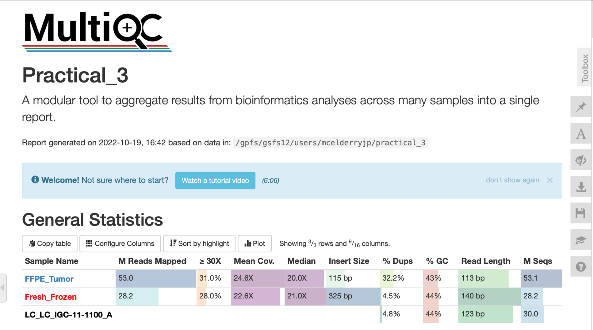
Above is the general statistics section of our MultiQC report. This section provides an overall summary of the most important statistics for our samples. These statistics are aggregated from the other QC reports generated by our script.

There is lots of information already contained within this general statistics section. Already we can see that the frozen tumor sample has similar coverage to the FFPE tumor, but has larger insert sizes, slightly longer read length, and much less sequence duplication. Our germline sample from frozen tissue has similar read length and duplication rate to the frozen tumor.

For Advanced Users: Just above these statistics, users can configure exactly which statistics to include in the summary table using the ‘Configure Columns’ button, can generate custom plots using the ‘Plots’ function, and can change the appearance of the entire report using the toolbox on the right of the screen. It is certainly worth exploring these functions on your own, but for the sake of time we won’t discuss them here.

Reviewing FASTQ-based QC results

9. We’ll begin by examining the FastQC output. Here is the command we used to run FastQC in our script:

## Run fastqc on all fastq files
fastqc -t $CPUS_PER_COMMAND -o $OUTDIR/fastqc_out \
$PATH_TO_PRACTICE3/sample_data/germline_EAGLE_WES/LC_LC_IGC-11-1100_A.bam \
$PATH_TO_PRACTICE3/sample_data/Fresh_Frozen/Fresh_Frozen.bam \
$PATH_TO_PRACTICE3/sample_data/FFPE/FFPE_Tumor.bam

Fastqc will generate a graphical quality report for each input sample (which can be in fastq or bam/sam/cram format), which it will title [sample name]_fastqc.html.

MultiQC has already incorporated these reports for us, so let’s examine them. Click on the ‘FastQC’ tab in the table of contents on the left to jump there.

Sequence Counts and Duplication

10. This first FastQC plot gives us an idea of how many sequences are in each sample, and also the level of duplication in each sample.

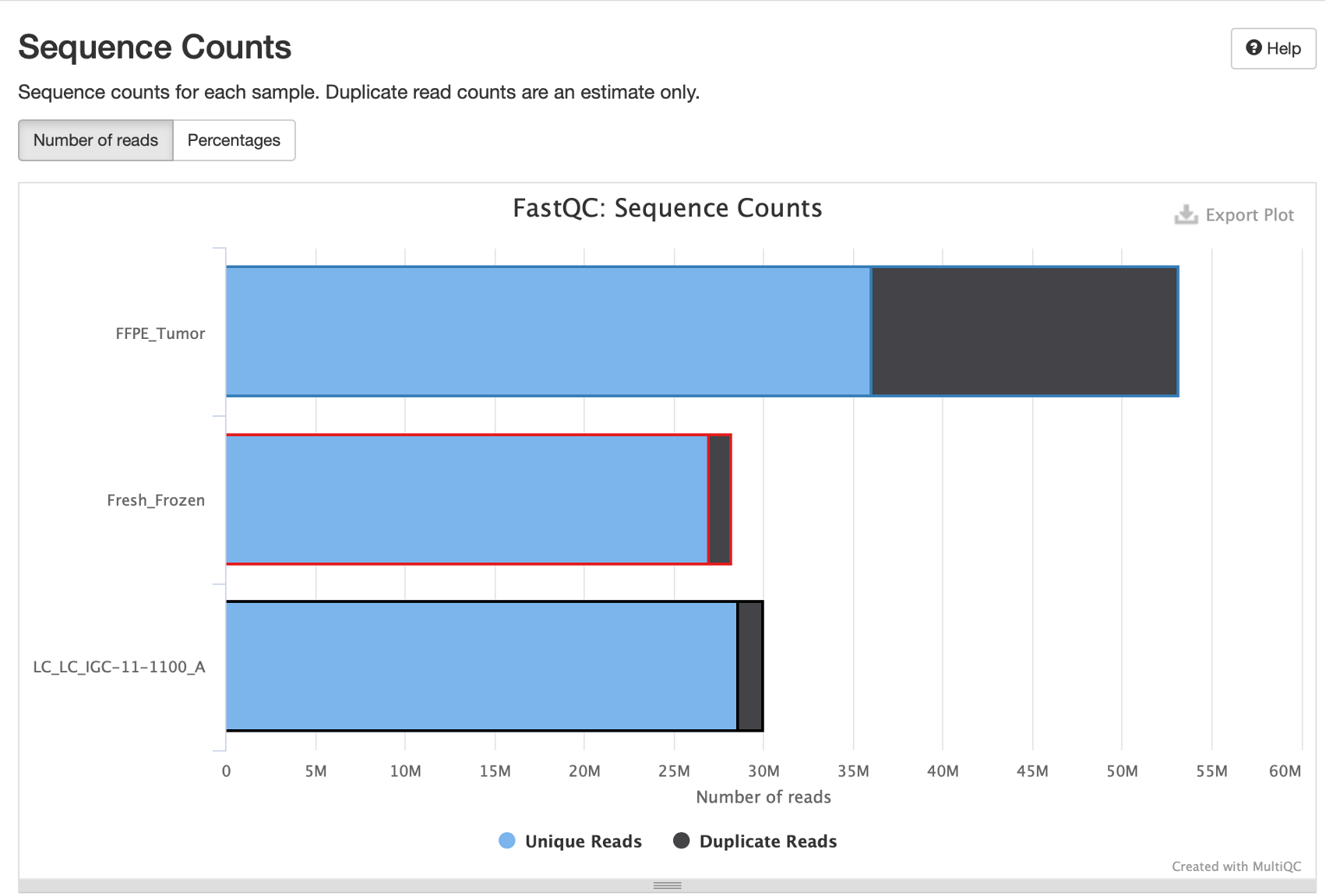
Hover over each of these bars and you’ll see that the FFPE tumors have more reads, but over 30% of those reads are duplicates.

11. Question: Why does the FFPE sample have a high duplication rate?

Answer: FFPE samples in general tend to have higher duplication due to DNA degradation and fragmentation. This leads to less diverse sequence libraries, and therefore higher duplication. Samples with moderate duplication and no other serious QC issues can still be useful provided you have adequate sequencing depth and coverage after excluding duplicates.

Sequence Quality and Adapter Content

12. Following the ‘Sequence Counts’ plot we have an important graphic showing the quality of sequences by position within the read.

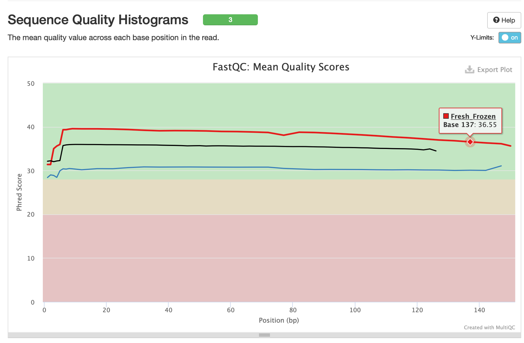
By hovering over these lines we can see that all of our samples are at or above median quality score 30 at every base position, and our frozen tissue samples are above 35. Quality score 30 is generally the minimum target for good quality sequencing, so all of our samples have acceptable sequencing quality (though you will get more false-positive variants in the FFPE sample due to its lower-end quality). Reminder: quality scores represent the 10 ^-Q/10 probability that a base was called incorrectly (e.g., Q30=10 ^-30/10=10 ^-3=1/1,000 chance of an error).

Average quality is expected to gradually decrease towards the end of reads due to limitations of sequencing by synthesis. A very sudden drop in sequencing quality, however, could be indicative of issues with the sequencing run.

13. The last plot we’d like to highlight is the ‘Adapter Content’ plot. This will show you what percentage of reads contain adapter sequences, per base position. Sequencing facilities will often do one pass of adapter trimming themselves before returning your data, but you may still have adapter content remaining. Here we can see that <5% of our germline frozen tissue reads contain adapter sequences.

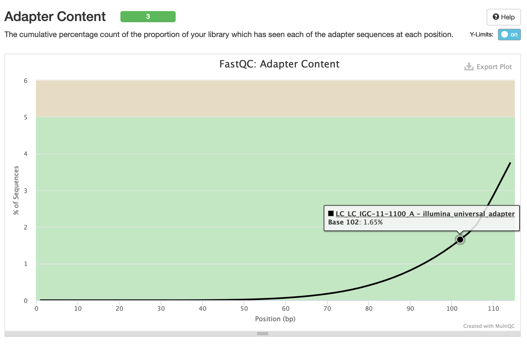
These adapter sequences can only negatively impact our analysis so they should be removed. We will remove these via read trimming.

Our two tumor samples are absent from this graph because they were already trimmed and no longer have adapter content. Generally speaking, untrimmed reads from FFPE samples will have more adapter content than frozen tissue due to smaller insert sizes (more on this later).

Read Trimming

14. Looking back at our submitted script, you will see just below our fastqc command we’ve submitted a job to run Trimgalore. Trimgalore will recognize and remove adapter sequences (either from a standard database by default, or as specified by the user) and also trim low quality bases from the ends of reads. Here is the command we ran in our script:

## Perform adapter/low quality base trimming on smaller fastq samples
trim_galore -j $CPUS_PER_COMMAND --fastqc --paired --gzip --stringency 3 \
-o $OUTDIR/trimgalore_out --basename trimmed-LC_LC_IGC-11-1100_A \
$PATH_TO_PRACTICE3/sample_data/germline_EAGLE_WES/LC_LC_IGC-11-1100_A.bam.fq1.gz \
$PATH_TO_PRACTICE3/sample_data/germline_EAGLE_WES/LC_LC_IGC-11-1100_A.bam.fq2.gz

Click to learn more about Trimgalore.

15. If you check the folder trimgalore, you will see the fastqc reports trimmed-LC_LC_IGC-11-1100_A_val_1_fastqc.html and trimmed-LC_LC_IGC-11-1100_A_val_2_fastqc.html. If you check these new fastqc reports on your local computer (download the reports here) and scroll to the adapter content graphic, you’ll see our samples no longer have adapter sequences.

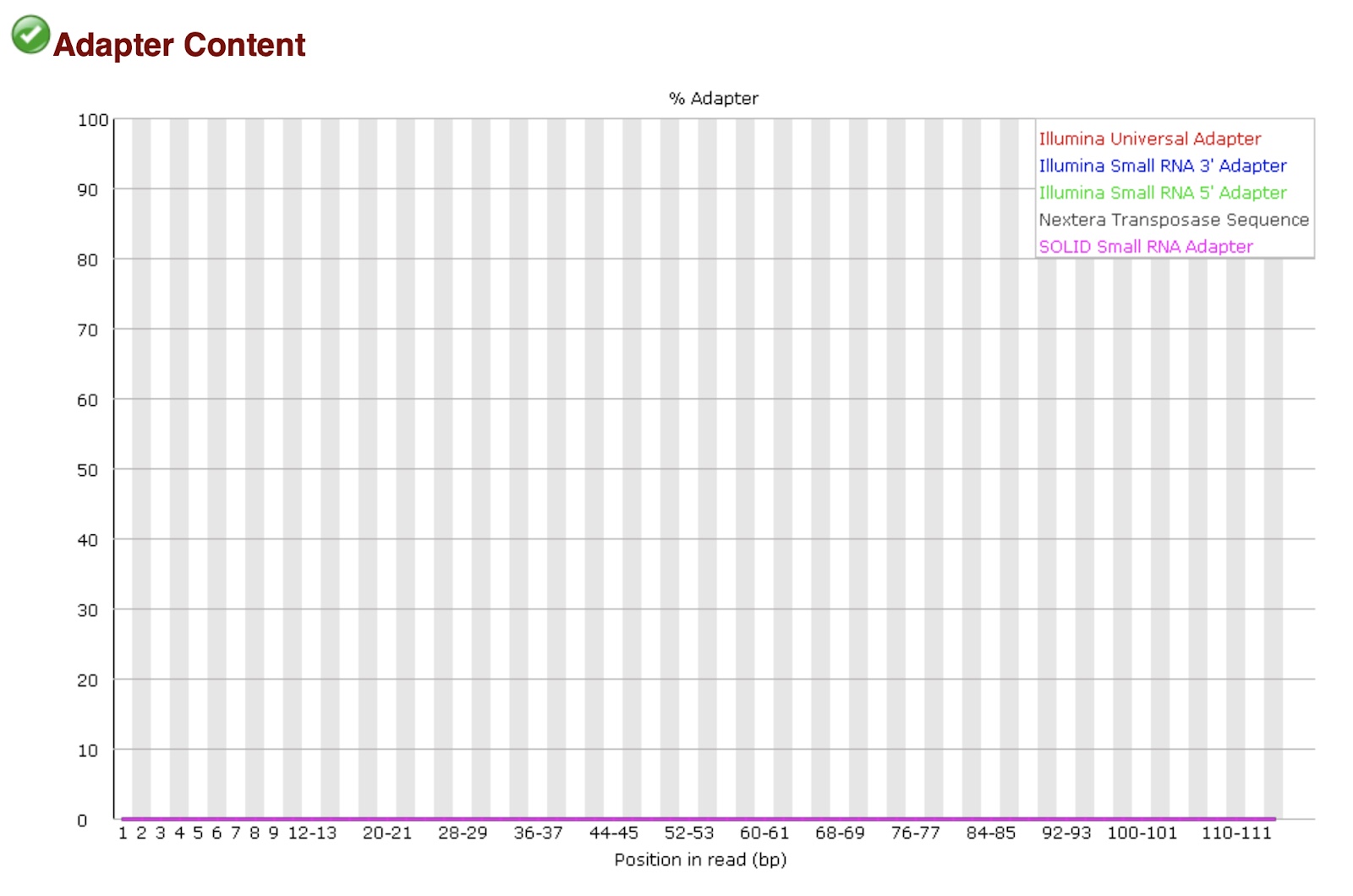
Note: you could also get this information from MultiQC, but lack of adapter content is more visually obvious in the original FastQC report.

Reviewing alignment-based QC results

After trimming your sequences (if necessary for your samples), the next step in a typical workflow is to align your sequences to a reference genome. Alignment is an hour(s) long, computation-intensive process that may also include additional re-alignment steps, duplicate sequences removal, and more.

We don’t have time for that in this practical, so we will instead focus on the quality control that comes after alignment. For those interested in learning more about alignment, we will instead refer you to this short tutorial. We will also briefly discuss alignment in session 4.

Alignment Flags with Samtools Flagstat

16. Just after the trimgalore command we ran the Samtools module ‘flagstat’.

## Calculate alignment flag statistics using Samtools
samtools flagstat -@ $CPUS_PER_COMMAND \
$PATH_TO_PRACTICE3/sample_data/Fresh_Frozen/Fresh_Frozen.bam > $OUTDIR/samtools_out/Fresh_Frozen.flagstat.txt &

samtools flagstat -@ $CPUS_PER_COMMAND \
$PATH_TO_PRACTICE3/sample_data/FFPE/FFPE_Tumor.bam > $OUTDIR/samtools_out/FFPE_Tumor.flagstat.txt

If you will recall, we actually ran this tool once already in practical 1. This tool will collect data on the alignment flags in our data to give us a simple view of how well our sequences mapped. If you need a refresher on alignment flags, see here.

17. To find this module in our MultiQC report, click on the Samtools tab in the table of contents on the left.

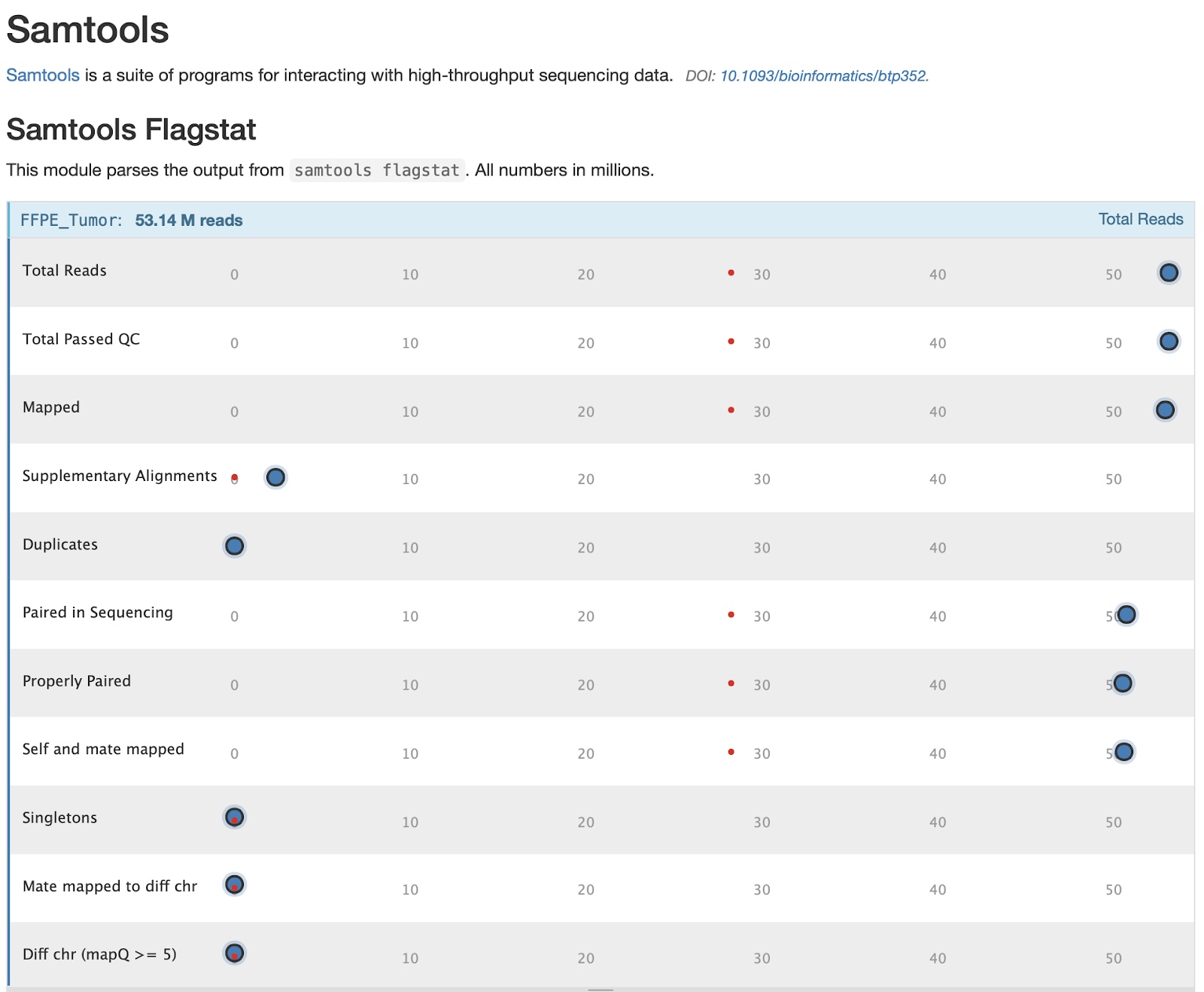
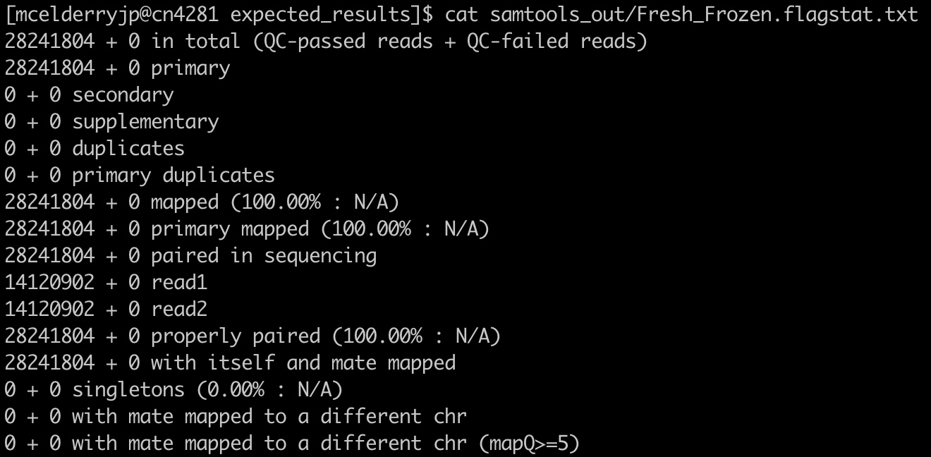
We can see the data for each sample by hovering over the points in the graphic. We’ll choose to focus on the FFPE sample for this module as it has some features worth noting. You can also examine the text version generated directly from samtools by opening the files ‘FFPE_Tumor.flagstat.txt’ and ‘Fresh_Frozen.flagstat.txt’.

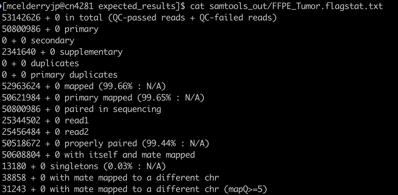
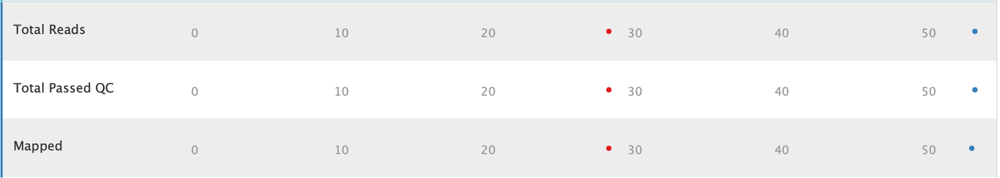
18. The first three stats give important information: how many reads were in each sample, how many reads passed QC (this is determined by the sequencer/sequencing facility), and how many reads mapped. In our case no reads failed QC, and almost every read in both samples mapped. Hover over the points to get specific numbers at the top of the table

19. Further down this table we have some statistics on how paired reads mapped:

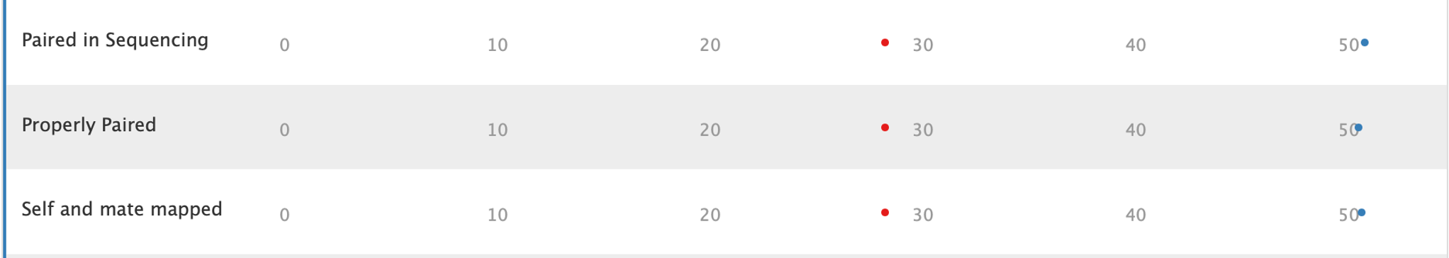
The take away from these stats is how many reads were paired, and how many pairs mapped properly (near one another in the genome and with expected stranded-ness). Most reads were properly paired in both samples which is good. A small number of reads may be improperly paired due to structural variants, but this should be a small fraction of total reads. The vast majority of reads are expected to be properly paired.

20. One notable stat for our samples is that the FFPE tumor has quite a few supplementary alignments:

When a sequencing read could be aligned to two or more distinct regions of the genome with no overlap, this is called chimeric alignment. One of the alignments is arbitrarily designated the “representative alignment” and the others are called “supplementary alignments”. Chimeric alignments can be indicative of structural variations.

However, for FFPE samples, chimeric reads could be artificially generated as part of the sequencing artifacts that can arise from the significant damage to DNA. Another possible reason for the higher number of supplementary alignment is that FFPE samples have shorter insert size, therefore their sequencing reads could potentially be mapped to more than one distinct region of the genome.

Additional care should be taken into account when using FFPE samples for calling structural variants. Additional information about this could be found here.

Assess Insert Sizes with Picard

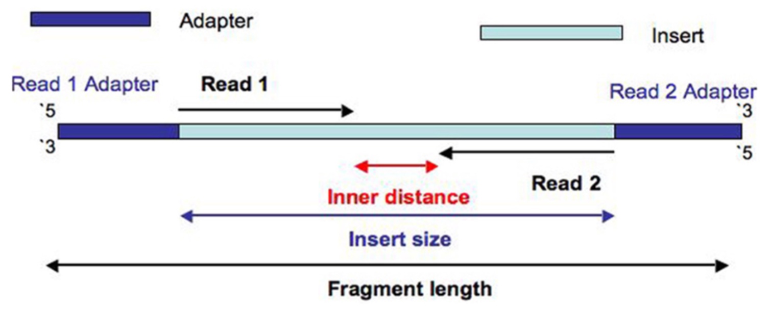
21. Let’s now turn to the output from the Picard module ‘CollectInsertSizeMetrics’. This tool, as the name implies, calculates insert size of our reads. Insert size and read length sound similar, but refer to different concepts. The insert size is the total length of the DNA fragment between the adapters, whereas the read lengths are the number of base pairs being sequenced in read 1 or read 2.

The command we used to generate this output in our script looks as follows:

## Calculate distribution of insert sizes with Picard
java -Xmx3g -jar $PICARDJARPATH/picard.jar CollectInsertSizeMetrics \
-I $PATH_TO_PRACTICE3/sample_data/Fresh_Frozen/Fresh_Frozen.bam \
-O $OUTDIR/picard_inserts_out/Fresh_Frozen.inserts.txt \
-H $OUTDIR/picard_inserts_out/Fresh_Frozen.inserts.pdf &

java -Xmx3g -jar $PICARDJARPATH/picard.jar CollectInsertSizeMetrics \
-I $PATH_TO_PRACTICE3/sample_data/FFPE/FFPE_Tumor.bam \
-O $OUTDIR/picard_inserts_out/FFPE_Tumor.inserts.txt \
-H $OUTDIR/picard_inserts_out/FFPE_Tumor.inserts.pdf

22. Let’s examine this report in MultiQC by clicking on ‘Picard’ in the left table of contents. Hover your mouse over the lines to see the samples they correspond to and the number of sequences at each insert size.

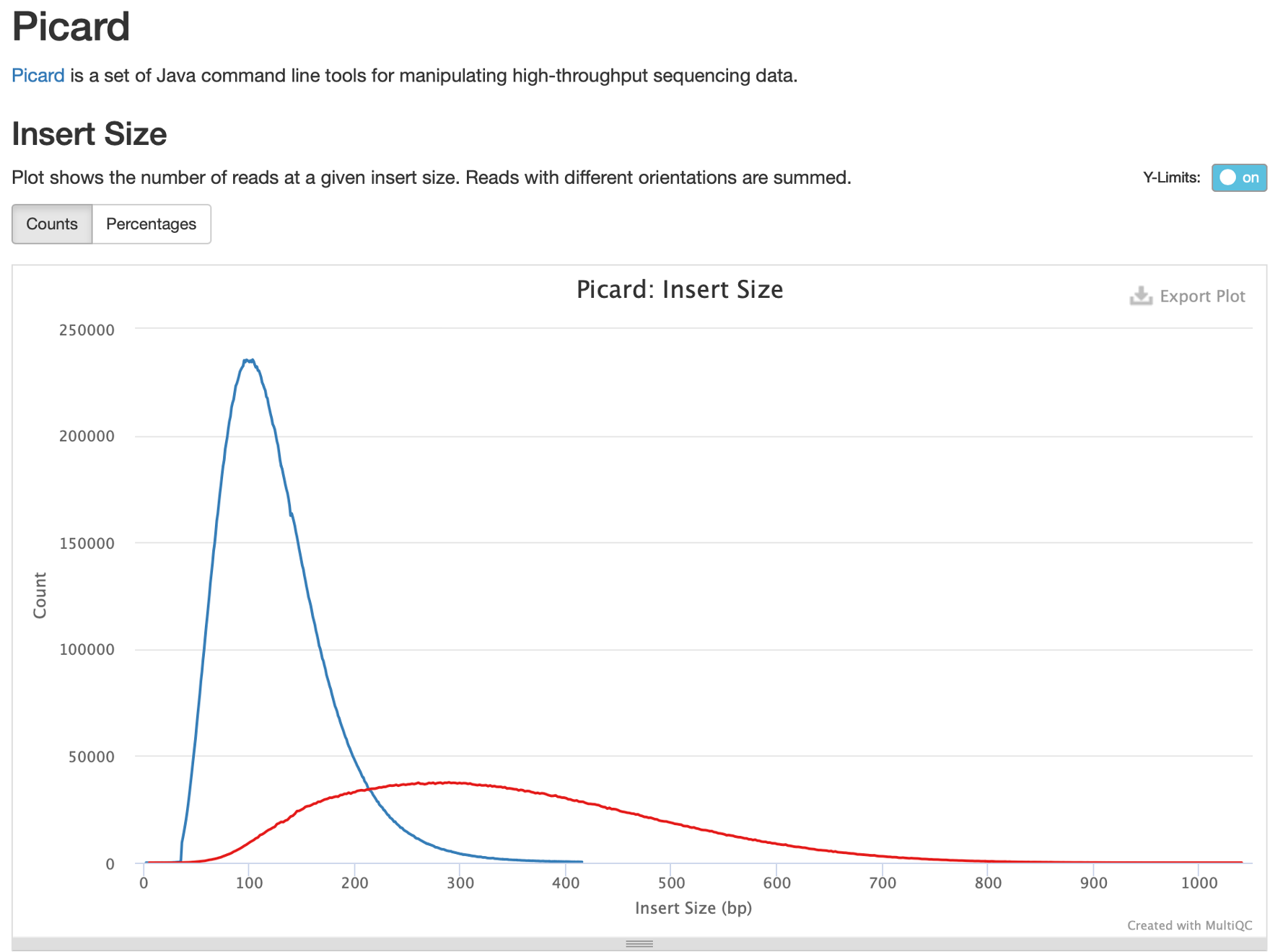
One difference that’s very obvious is that the FFPE samples all have relatively small insert sizes, peaking at around 101bp. This is smaller than our average read length of 113bp, and means that most paired reads in this sample totally overlap, like so:

As a result the effective sequencing depth for this FFPE tumor is therefore roughly half of the estimated overall depth as both reads in most pairs contain the same information.

Small insert sizes in this case are due to DNA degradation as a result of the FFPE process. Small insert sizes will also cause:

• higher adapter content and decreased read length*
• increased duplication rate
• make it difficult to discover and resolve structural variants or rearrangements
• possibly cause false positives during variant calling
• possibly impose other discovery limitations depending on your study design.

By contrast, the insert size distribution of the frozen sample peaks at ~300bp with a read length of 140bp. Do note that insert size also can be too large; if your inserts are many times larger than your sequencing length this could reduce evenness of coverage.

Insert sizes should ideally be a little larger than 2x read length. A good distribution of insert size for short read WES and WGS data is therefore a strong peak around 300-500bp.

* Note: you may recall that although we just said FFPE samples often have more adapter content, we didn’t observe any adapters in this FFPE sample with FastQC. This is because the fastq samples for this FFPE tumor were already adapter trimmed.

Calculate Genome Coverage with Mosdepth

The last QC metric we will discuss is sequencing coverage over the genome. Coverage can be roughly defined as the number of sequencing reads that sequence, or “cover”, each base in the genome.

In addition to learning how evenly your sequencing covers the genome, you can also check the sex of your sample using per-chromosome coverage statistics. This will allow you to verify the integrity of your sample by comparing the observed sex to the expected sex of the sample.

23. To do this we ran the tool mosdepth in our script:

## Calculate sequencing depth for both samples, isolating only the parts of the genome covered by the exome capture kit
mosdepth -t $CPUS_PER_COMMAND \
-b $PATH_TO_PRACTICE3/references/sorted-SeqCap_EZ_ExomeV3_Plus_UTR_hg19_primary_annotated.bed \
$OUTDIR/mosdepth_out/FFPE_Tumor $PATH_TO_PRACTICE3/sample_data/FFPE/FFPE_Tumor.bam &

mosdepth -t $CPUS_PER_COMMAND \
-b $PATH_TO_PRACTICE3/references/sorted-SeqCap_EZ_ExomeV3_Plus_UTR_hg19_primary_annotated.bed \
$OUTDIR/mosdepth_out/Fresh_Frozen $PATH_TO_PRACTICE3/sample_data/Fresh_Frozen/Fresh_Frozen.bam

The -b option in the mosdepth command is very important to note. Recall that the samples we analyzed were whole exome sequencing samples, thus it would be misleading to include non-coding regions of the genome in our coverage calculation. For that reason we’ve specified a BED interval file with -b to restrict the coverage calculation to only the regions of the exome which we targetted during sequencing. The BED file you use must be specific to the kit you use for exome capture prior to sequencing.

24. Now let’s examine the report in MultiQC by clicking on mosdepth in the table of contents.

From the general statistics table at the top of the report, we can see that the median coverage is ~21X for the frozen tumor and ~20X for the FFPE tumor.

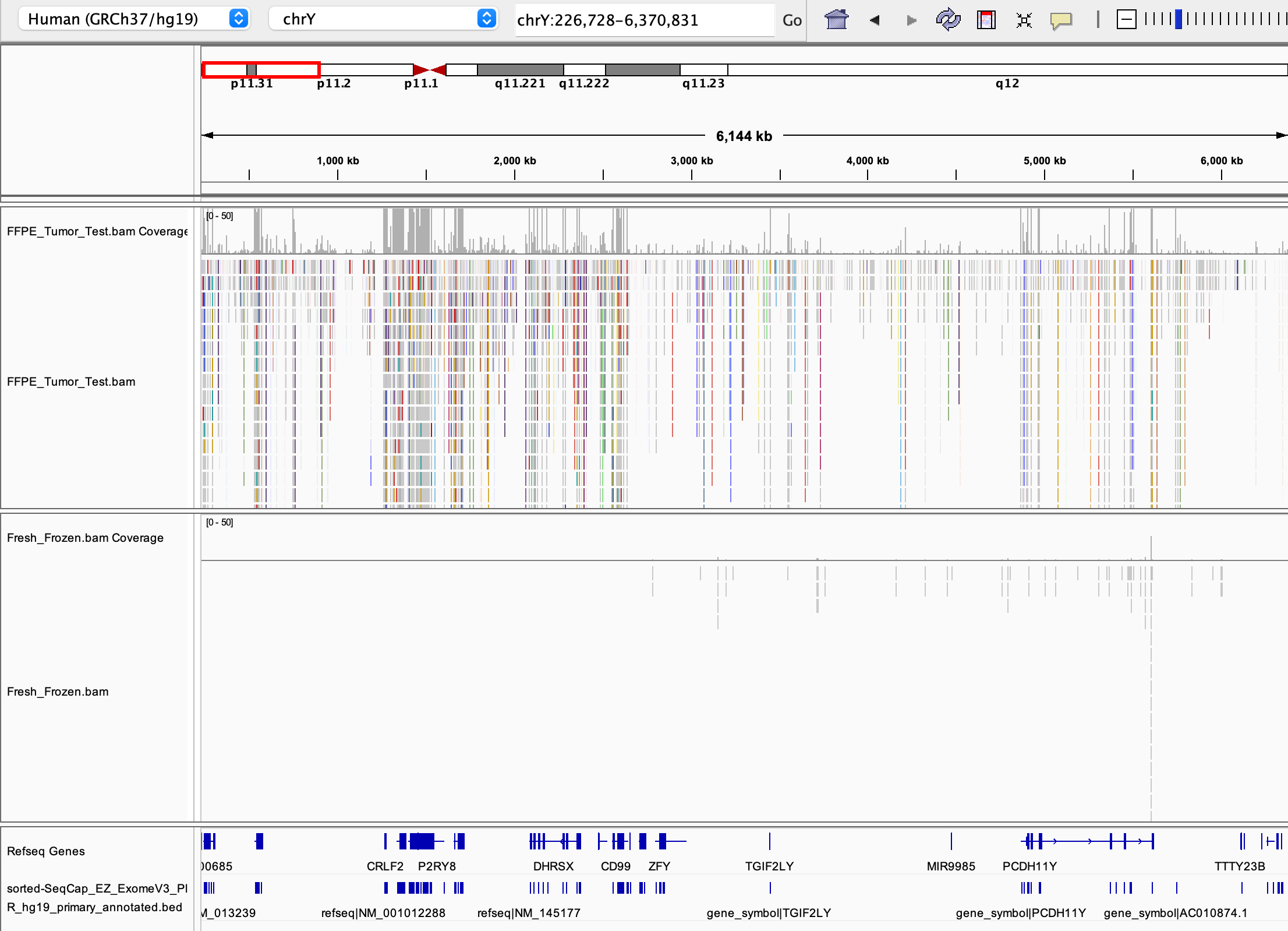
25. Now let’s look at the coverage per chromosome:

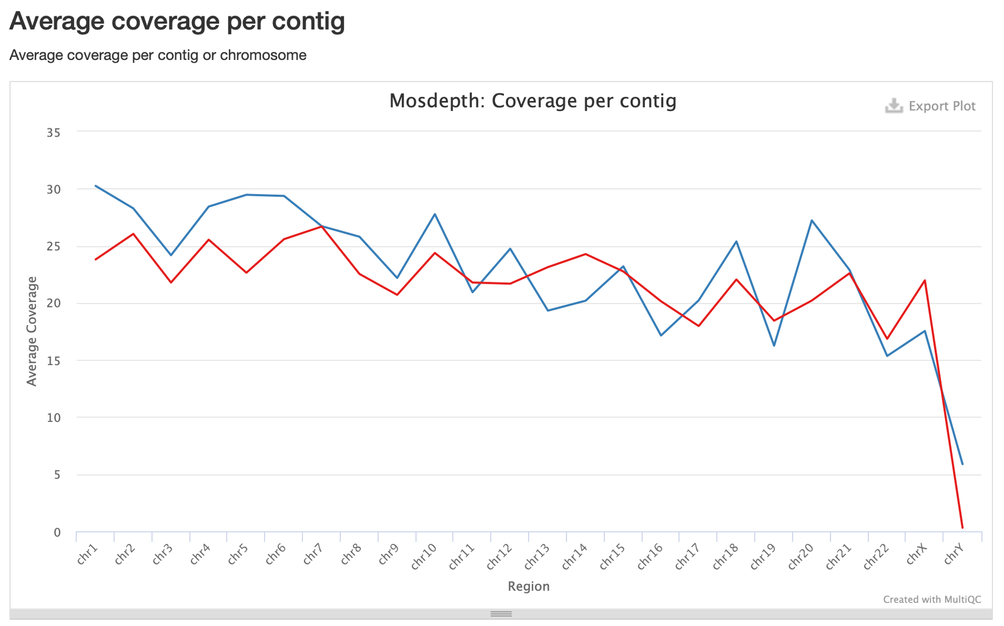
Here we can see that coverage fluctuates between chromosomes, but is consistently between 20-30x. Note the sex chromosomes on the right: our frozen tumor has virtually no coverage on the Y chromosome, which is consistent with the expected sex of this sample (female). The FFPE sample, however, is more ambiguous with ~17.5X coverage of the X chromosome and ~6X coverage of the Y chromosome.

26. Question: Records indicate this FFPE sample was derived from a female sample, so why does this sample have coverage of the Y chromosome?

Answer: There are two possible reasons. One is that the FFPE sample has been cross-contaminated or swapped with a sample from a male individual. Additional QC can verify this by estimating the intersample contamination rate (e.g., VerifyBamID). The other possibility is incorrect mapping to chromosome Y, particularly from low quality reads. This is especially likely on chromosome Y due to its complex features (lower mappability, many repeat regions, high proportion of heterochromatin structure, etc.). This can occur even in uncontaminated female samples. A more strict approach is necessary in these cases.

Assess Sex Concordance with Somalier

At the end of our script we ran the tool Somalier. Somalier calculates a relatedness score between samples using a list of common SNPs, which can be useful for identifying related individuals and sample swaps. Additionally, Somalier calculates a few useful statistics for sex concordance, namely zygosity of chromosome X SNPs.

27. The Somalier commands are at the end of this script and require running ‘somalier extract’ on each sample to extract SNP information, followed by ‘somalier relate’ to calculate relatedness and other statistics between samples.

## Run somalier - this program is not installed on Biowulf, for future use you must download here:
## https://github.com/brentp/somalier/releases
$PATH_TO_PRACTICE3/algorithms/somalier extract -d $OUTDIR/somalier_out/ \
-s $PATH_TO_PRACTICE3/references/sites.hg19.vcf.gz \
-f $PATH_TO_PRACTICE3/references/hg19_canonical_correct_chr_order.fa \
$PATH_TO_PRACTICE3/sample_data/FFPE/FFPE_Tumor.bam &

$PATH_TO_PRACTICE3/algorithms/somalier extract -d $OUTDIR/somalier_out/ \
-s $PATH_TO_PRACTICE3/references/sites.hg19.vcf.gz \
-f $PATH_TO_PRACTICE3/references/hg19_canonical_correct_chr_order.fa \
$PATH_TO_PRACTICE3/sample_data/Fresh_Frozen/Fresh_Frozen.bam &
wait

$PATH_TO_PRACTICE3/algorithms/somalier relate -o $OUTDIR/somalier_out/somalier \
$OUTDIR/somalier_out/FFPE_Tumor.somalier \
$OUTDIR/somalier_out/Fresh_Frozen.somalier

28. Somalier has been included in our MultiQC report. Click on Somalier in the table of contents, but note that we won’t look at the automatically generated plots (these plots mostly show relatedness which is useful for larger studies but not relevant for this use-case).

29. Instead, just above the Somalier summary statistics table click on the ‘Plot’ option:

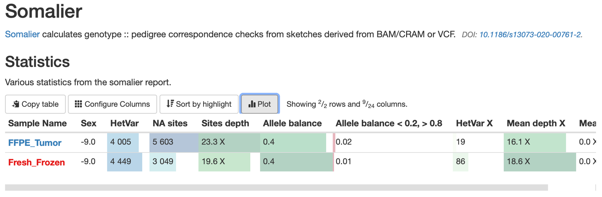
30. In the window that appears, select ‘HomAltVarX’ and ‘HetVarX like so.’

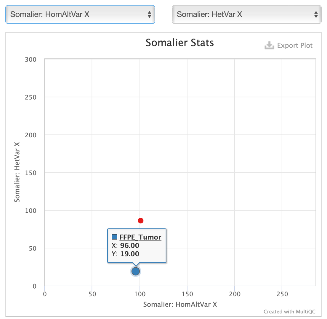
Here we can see that our FFPE tumor has very few heterozygous SNPs on the X chromosome, which is unusual for a female with two X chromosomes. Compare this to the fresh frozen tumor where the ratio of heterozygous and homozygous SNPs is roughly 50/50. In combination with relatively high chromosome Y coverage in the FFPE tumor, this is strong evidence for a contamination issue.

Indeed, examine the image below captured from IGV (Integrated Genomics Viewer); visualizing the alignment for this sample shows consistent, exome-specific coverage on the Y chromosome in the FFPE tumor sample, but no coverage in the frozen sample (the histograms in the middle of the image). This indicates that false-positive mapping is an unlikely explanation for the observed Y chromosome coverage.

(NOTE: Somalier will also assess X and Y coverage, but it calculates this coverage using the provided SNPs; unless all of these SNPs are in the exome the coverage calculation will be inaccurate for WES).

Summary of the Effect of FFPE on NGS Quality

As noted throughout this practical FFPE samples often have several quality issues, such as a high proportion of PCR duplicate reads and very short insert sizes. Consequently the overall coverage, without duplicates and considering the overlap between two paired reads, should always be calculated to determine if you have enough depth. A high proportion of PCR duplicates can be an indication that your starting DNA was highly fragmented, and you may also observe a higher number of artifacts during variant calling. Samples with an extremely high PCR duplicate rate may have to be excluded if the depth of coverage (without PCR duplicates) is too low. A high proportion of unmapped reads is also a red flag, as well as a high proportion of mates mapped to a different chromosome.

Additional QC at the variant level and a strict bioinformatic post-processing of the variant calling are both strongly recommended when analyzing FFPE samples. We will cover this in Session 4: Mutation Calling and Analysis.

OPTIONAL: Sequencing Strategy-specific QC Metrics

The previous QC metrics we’ve introduced are useful for almost any NGS application, regardless of study design and sequencing methodology. Now we will focus on QC metrics that are particularly suited or only applicable to certain experimental designs.

Targeted Sequencing and Whole Exome Sequencing

The intent of targeted and exome sequencing is to focus your sequencing efforts on a relatively small area of the genome expected to have the greatest importance to your disease of interest. Thus it’s useful to know how well you sequenced your target region(s), and how much of your sequencing was off target.

31. This is something we can answer using another function of Picard, ‘CollectHsMetrics’ (Collect Hybrid Selection Metrics). Here’s an example for how to do this:

## 002 Running picard CollectHsMetrics
java -Xmx8g -jar $PICARDJARPATH/picard.jar CollectHsMetrics \
I=$PATH_TO_PRACTICE3/sample_data/FFPE/FFPE_Tumor.bam \
O=$PATH_TO_PRACTICE3/0-Off-Targeted/scr-0-Off_Targeted-Output/FFPE_output_hs_metrics.txt \
R=$PATH_TO_PRACTICE3/references/hg19_canonical_correct_chr_order.fa \
BAIT_INTERVALS=$PATH_TO_PRACTICE3/0-Off-Targeted/sorted-SeqCap_EZ_ExomeV3_Plus_UTR_hg19_primary_annotated.interval_list \
TARGET_INTERVALS=$PATH_TO_PRACTICE3/0-Off-Targeted/sorted-SeqCap_EZ_ExomeV3_Plus_UTR_hg19_primary_annotated.interval_list

This code is included at the end of our script in comment form, and the outputs can be found in the Picard-CollectHsMetrics/ folder of our practical 3 resources folder (/data/classes/DCEG_Somatic_Workshop/Practical_session_3/).

The BAIT_INTERVALS and TARGET_INTERVALS are two subtly different genome interval files; the targets are the exact intervals corresponding to the areas of the genome you wanted to sequence (e.g. gene TP53) and the baits include those targets, plus any extra bases in the DNA baits used for exome target/capture (e.g. small overhangs up and downstream of a target). CollectHsMetrics requires both to be specified, but for most cases it’s perfectly fine to use a single target file for both.

32. Let’s examine the output with ‘less Fresh_Frozen_output_hs_metrics.txt’:

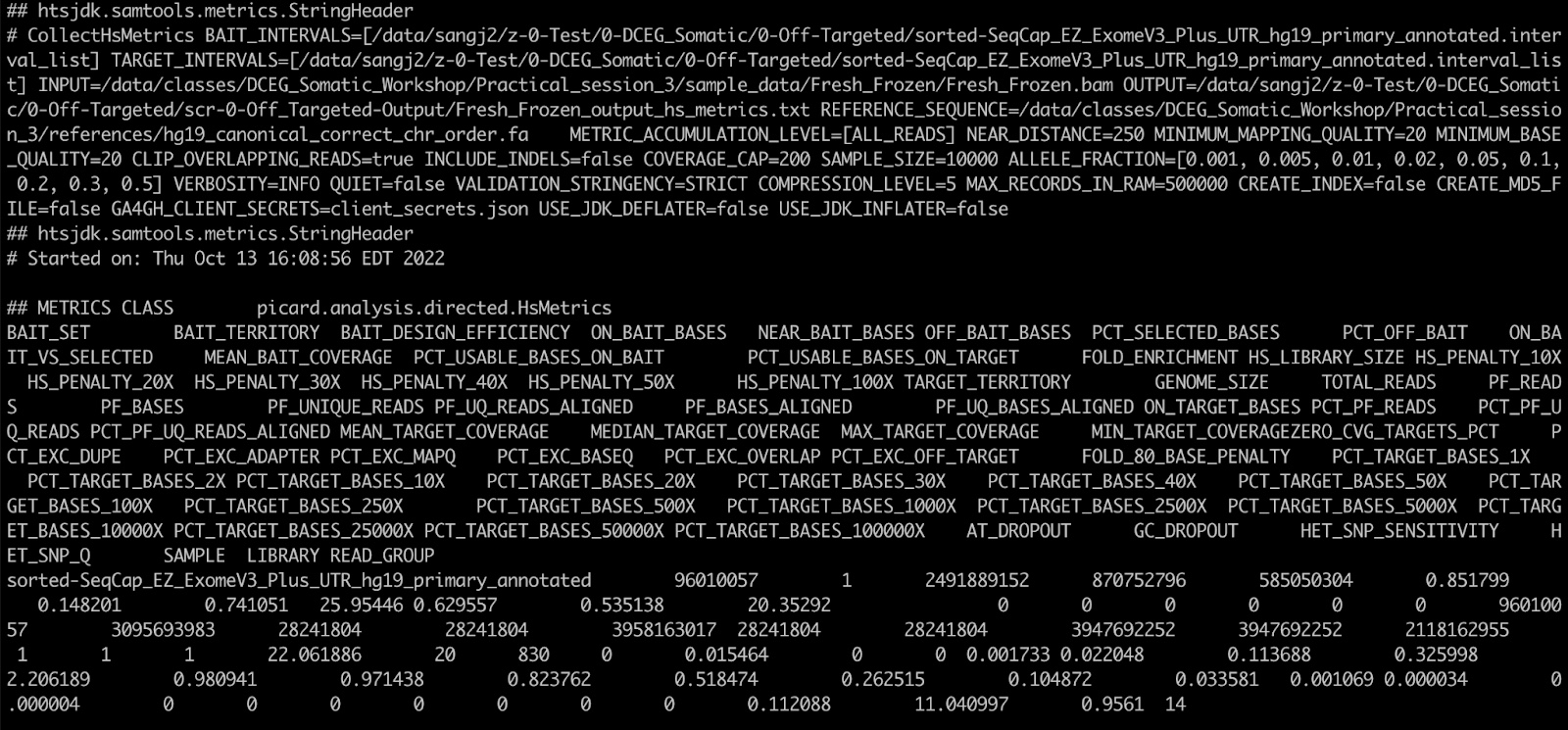
Since this returns a rather lengthy and hard-to-read report, we will extract the pieces of information we need with ‘cut’, which extracts columns of data that we request by column number.

33. First quit less with :q, then enter the following:

grep -A 2 "## METRICS" Fresh_Frozen_output_hs_metrics.txt | tail -2 | cut -f 46,44,48,49,50

The stats we’re looking at in order are the percentage of off-target sequences expressed in units of base pairs, followed by the percent of target bases covered at least 1x, 10x, 20x, and 30x. In this fresh frozen tumor, ~32% of sequenced bases fell off target, however, we do still have at least 1x coverage over 98% of our target and 10x coverage over 82% of the target. If we examine the FFPE tumor, we’ll see it has less off-target sequencing but slightly less even target coverage as well.

IGV

IGV is an extremely useful resource for visualizing the alignment in areas of any genome and is very commonly used for manually verifying the results of bioinformatics algorithms.

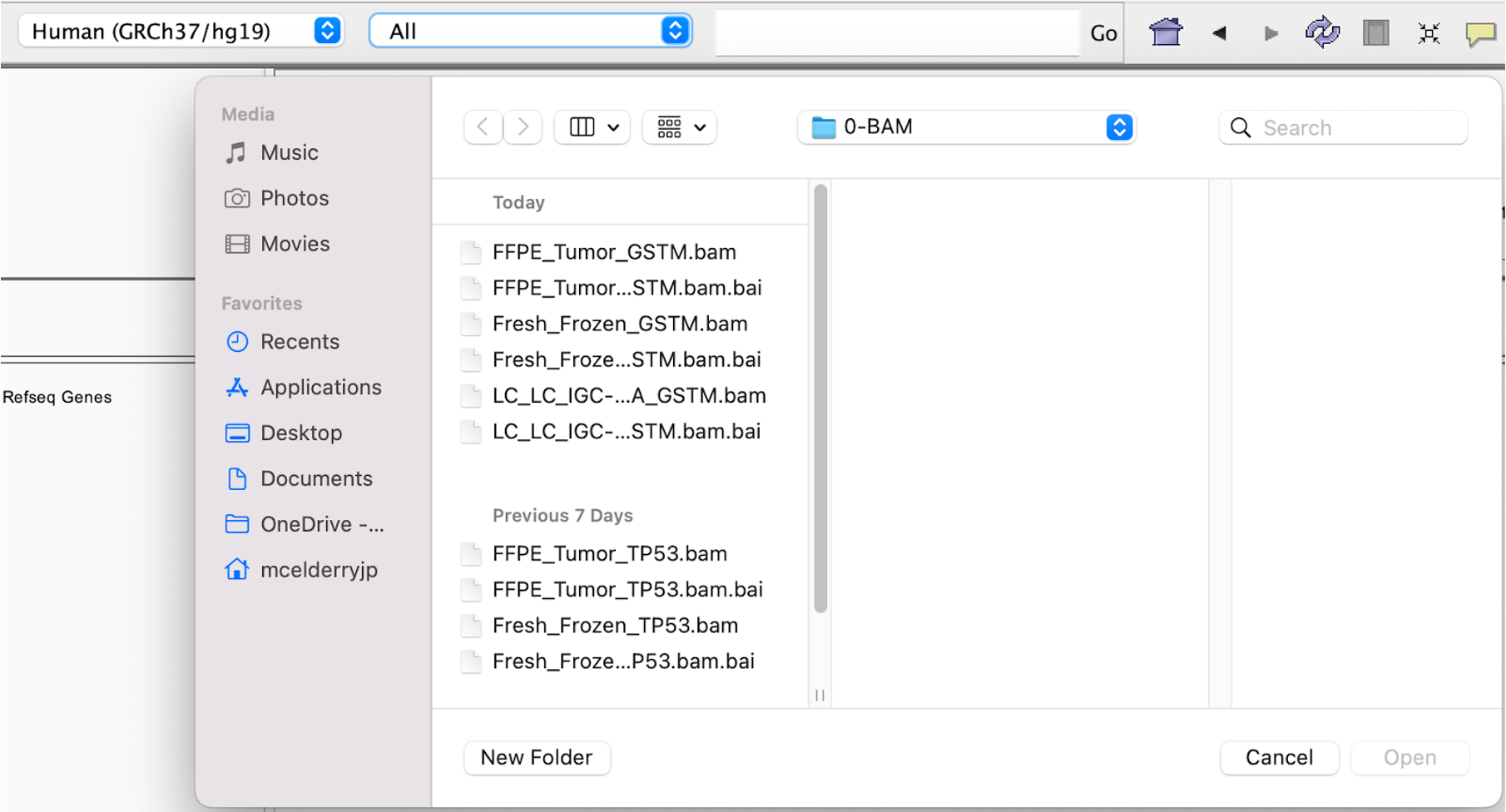
34. Since we will use IGV locally on your computer (i.e. not on Biowulf), you’ll need the alignment files on your computer. Rather than download from Biowulf, please download the bam files we’ve prepared here, which have been isolated to only the region around GSTM1 and GSTM2 using samtools view.

35. Once that’s done, open IGV on your local computer and follow these steps:

• Ensure that the genome selector in the top left is set to ‘Human (GRCh37/hg19)’. If not, click that selector, click on ‘More…’, and then select ‘Human (hg19)’ and hit ‘OK’.
• Click File in the top left and click “Load from File”.
• Locate and open the files Fresh_Frozen_GSTM.bam, FFPE_Tumor_GSTM.bam, and LC-LC-IGC-11-1100_A_GSTM.bam which we’ve downloaded, as well as the exome annotations BED file for our exome capture kit

36. This should now open our samples in the viewer, though you won’t actually see any data until you pick somewhere in the genome to zoom in. Let’s zoom in on GSTM1 to see what alignments look like. To do this, enter ‘GSTM1’ into the box at the top.

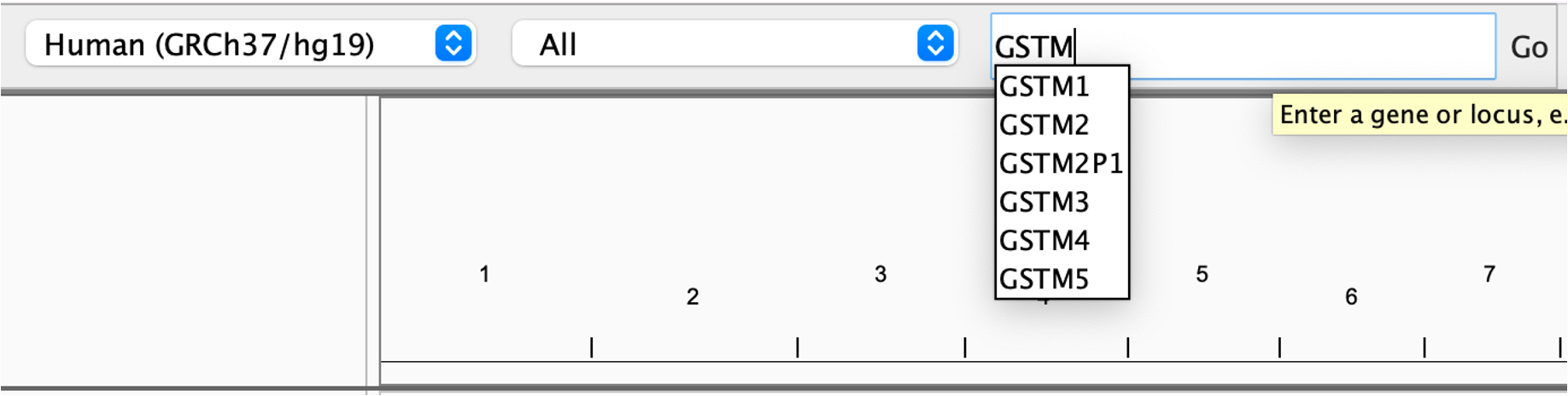
This will automatically search for genes matching this pattern. Click GSTM1 to automatically jump to GSTM1 in the genome browser.

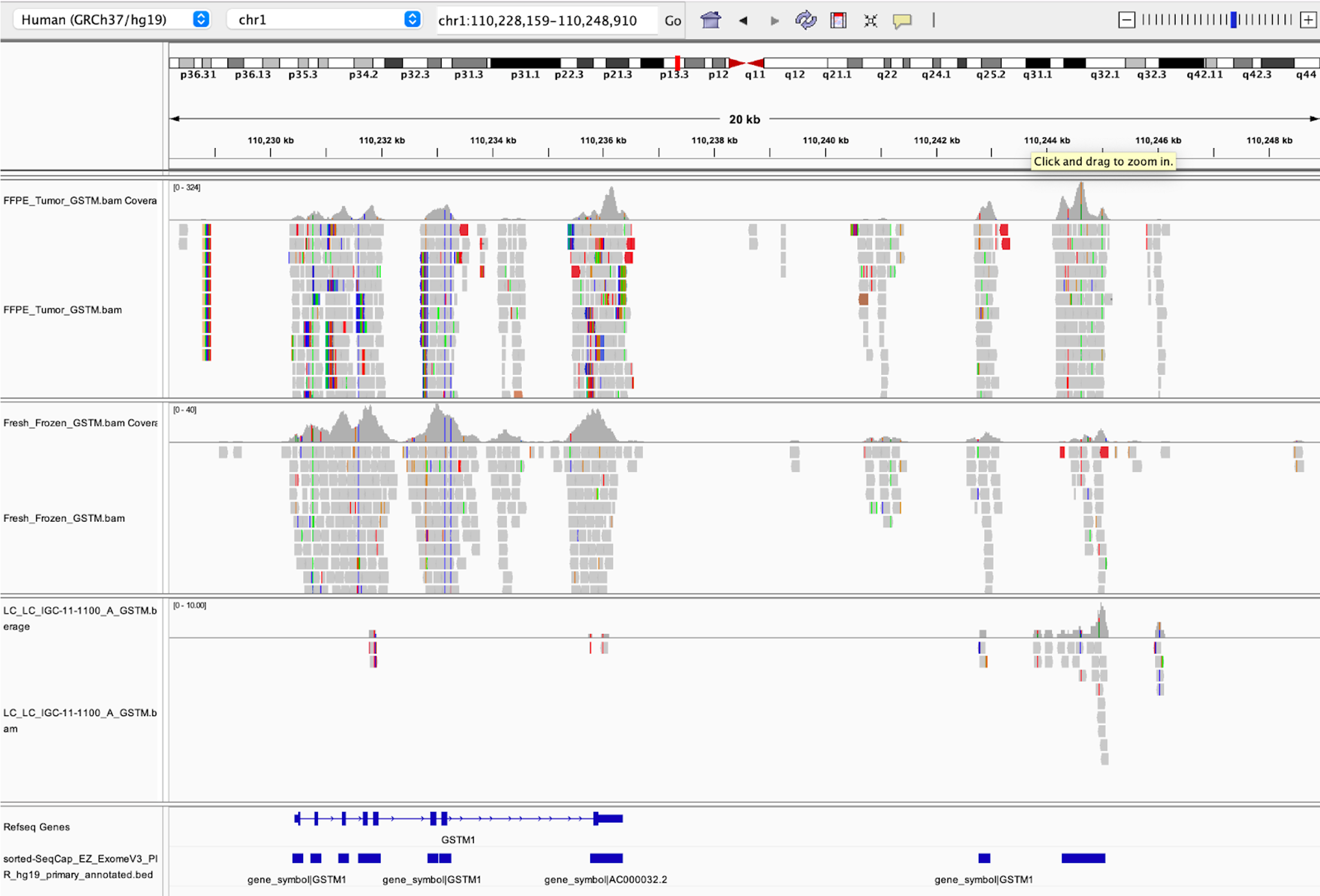
• Look at the bottom of the screen, specifically the blue rectangles. The first track of blue rectangles corresponds to the Refseq Genes annotation, and importantly the second track of blue rectangles are the regions of the genome being sequenced by our exome kit.
• In the middle of the screen, the gray rectangles correspond to our sequencing reads and the histogram above those reads is a representation of the depth of sequencing per base position. From this graph you can see that our sequencing data lines up well with the capture regions of our exome kit.
• You can also see that the third sample has a distinct lack of coverage over GSTM1. This is a strong indicator of a deletion in this sample.

When you encounter unexpected or surprising results, or you just want to verify the results from an algorithm, using IGV to visually examine the alignment is often one of the first steps taken as a sanity check. You may find that the region of the genome in question is highly repetitive, has some other unique feature affecting your algorithm, or the reads mapping to the region do not actually map very well.

Whole Genome Sequencing

Based on our Sherlock-Lung study, we recommend several additional steps for quality control of whole-genome sequencing data. We will discuss some of these analyses in future sessions.

• We suggest removing any tumor samples with median sequencing depth less than 40x and removing any normal samples less than 25x. These thresholds will allow sufficient read depth for detecting somatic variants with enough germline reads as a control.
• Cross-sample contamination can be identified using genotype concordance. This can be done with Conpair or VerifyBamID. We recommend removing any sample with a contamination level above 5%.
• For non-family studies, we keep only one subject with high tumor sequencing depth if two samples from different subjects have relatedness >0.25. The relatedness among all subjects can be estimated with Somalier. We also use Somalier to screen for labeling issues among tumor-normal pairs (e.g., mislabeled IDs).
• If many large copy number events are observed in normal samples, as detected by SCNA algorithms (e.g., Battenberg), this indicates tumor and normal samples may be swapped or mislabeled during sequencing. Paired tumor-normal samples may be reanalyzed by switching tumor and normal status.
• Mutational signatures can be used to infer cancer types or treatments. For example, in our Sherlock-Lung study, we observed some tumor samples with mutational signatures associated with ultraviolet light, and with platinum-based drug chemotherapy in untreated tumors. These are probable melanoma metastases and need to be removed for downstream analysis.
• For analysis of somatic alterations, tumors with low purity (e.g., <0.2) and few mutations (e.g. <100) should be removed. Additionally, for tumor evolution analysis it is important to estimate the number of reads per tumor chromosomal copy (NRPCC, see the reference here). We recommend including only tumor samples with NRPCC>10 for tumor evolution analysis.