MEGSA (Mutually Exclusive Gene Set Analysis)
Since we will not be going over the use of another tool, MEGSA, but we wanted to provide you with the material should you be interested in learning about this additional tool on your own time.
MEGSA is a R package used to identify mutually exclusive gene sets (MEGS). The purpose of identifying mutually exclusive gene sets (MEGS) is to help address the challenges that come with identifying driver genes and pathways. The two main challenges include:
- identifying infrequently mutated driver genes requires a very large sample size to achieve statistical significance
- investigation of relationships among mutated genes and the subsequent identification of oncogenic pathways can be complex (Hua et al, 2016).
Originally, ME analysis was for pairwise analyses, but as we know, cancer pathways typically involve multiple genes, and so the original pairwise analyses have been extended to identify MEGS instead. There are multiple methods that have been proposed for ME analysis, but each method is different from the next with regard to the statistical tests of the method and the search criterion used for identifying MEGS. The analytical framework of MEGSA is based on a likelihood ratio test and model selection procedure. This method can be used for de novo discovery, pathway-guided searches, and expanding established small MEGS. The expectation of MEGSA is that it can be useful for identifying oncogenic pathways and driver genes that would have been missed by frequency-based methods (Hua et al, 2016).
You can find the publication for MEGSA here. MEGSA was created through contributions by several researchers at the National Cancer Institute. The MEGSA package can be downloaded from the Division of Cancer Epidemiology and Genetics website: https://dceg.cancer.gov/tools/analysis/megsa. However, we recommend downloading the zip file below instead, because it includes the MEGSA files, a few pre- pre-generated files that will save you some run time, and a modified example R script from MEGSA.
This tutorial will show you how to use the example data included in the package, but with an abridged version of the data so that the analysis does not take so long.
1. If you haven’t already, download the zip file that contains all of the files necessary to use MEGSA, as well as the pre-generated files.
2. First, we will source the MEGSA.R file, which contains all of the necessary functions in the MEGSA package.
3. Then, we will load the mutation matrix included in the package, which includes binary mutation data for TCGA LAML samples.
mutationMat <- as.matrix(read.table("mutationMat_LAML.txt", header = TRUE, row.names = 1) != 0)
We will filter this data to include only specific genes, to minimize the time to get a result:
mutationMat_tmp <- mutationMat[,c('FLT3','TP53','KRAS','NRAS','PTPN11','KIT','RUNX1')]
Save this data frame in a file in case you need to use it later (Note: you would need this file for a command to run MEGSA all at the same time- see Additional Information).
write_delim(as.data.frame(mutationMat_tmp), file = 'mutationMat_tmp_example_byuser.txt', delim="\t")
Use this to read it back into R if necessary:
mutationMat_tmp <- as.matrix(read.table("mutationMat_tmp_byuser.txt", header = TRUE))
If you look at this data, you will see that there is a TRUE/FALSE value for each sampleID/gene pair, noting if there was a mutation or not in the gene for a given sample.
4. Next, we will run the permutations step to generate the distribution of the maximum LRT statistic under the null hypothesis. In this case, the null hypothesis is the idea that the set of genes in the mutation matrix (what we load in step two), contains no MEGS of any size. You can use the following command to run it yourself. Note: this step takes about 30 minutes to run on a local machine.
maxSSimu <- funMaxSSimu(mutationMat_tmp, nSimu = 1000, nPairStart = 10, maxSize = 6)
Or, read in the file already provided:
maxSSimu <- as.matrix(read.table("maxSSimu_example.txt", header = TRUE))
The following explain the parameters used:
nSimu: number of simulations (recommend 1000 or more, it may take ~ 10 hours for 1000 simulations).nPairStart: first tested all pairs of genes and then picked up the top nPairStart gene pairs (ranked by P-values) to perform multiple-path search to include more genes. IncreasingnPairStart: will slightly increase power but linearly increase the computational time.maxSize: the maximum size of putative MEGS.
5. Write your own file after running step 2 (if you did not use the maxSSimu_example.txt file provided to save some time) so that you do not have to run this step again in the future.
write_delim(as.data.frame(maxSSimu), file = 'maxSSimu_example_byuser.txt', delim="\t")
Use this to read it back into R if necessary:
maxSSimu <- as.matrix(read.table("maxSSimu_example_byuser.txt", header = TRUE))
6. Now we identify significant MEGS based on a significance level or family-wise error after multiple testing correction based on permutations. We use a level of 0.05 here:
resultMEGSA <- funSelect(mutationMat_tmp, maxSSimu, level = 0.05)

str(resultMEGSA)
This command will display a list of two components in the result output:
resultMEGSA$p: the global p valueresultMEGSA$MEGSList: a list of significant MEGS)
7. MEGSList is the list of significant MEGS. We can pull this from the resultsMEGSA object:
MEGSList <- resultMEGSA$MEGSList
You will see that we have 5 gene sets in the MEGSList object we created.
Each of these has four attributes:
S: LRT statisticpNominal: nominal p valuepCorrected: multiple-testing corrected p valuecoverage: the coverage of the MEGS)
We can look at these here, using the following:
str(MEGSList)
8. Then we can convert this list of MEGS to a data frame and export it:
MEGSDF <- funPrintMEGS(MEGSList, outputFile = "resultMEGS_example.txt")
9. Finally, we can visualize the MEGS and generate corresponding figures for each gene set:
funPlotMEGS(MEGSList, mutationMat, outputDir = "figure_example", type = "pdf")
10. There will be a pdf for every gene set identified. Here is an example figure (gene_set_1) and how to interpret it:
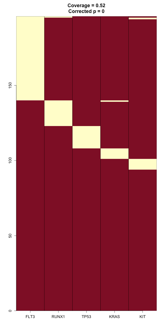
This gene set includes FLT3, RUNX1, TP53, KRAS, and KIT. This MEGS was identified in about half of the samples (52%), and its corrected p-value is 0. The yellow coloration denotes mutation, and the red denotes no mutation of a gene in a given sample. We can see that these mutations are almost always mutually exclusive from each other, except for in a few cases where a mutation in one gene overlaps a mutation with another gene. In relation to one of the aims of MEGSA, to allow for identification of driver genes even when mutation in the gene is infrequent, this shows that for example, KRAS is infrequently mutated in these samples, but is a well-known cancer driver gene. This is a driver that could have potentially been missed in these LAML samples if using a frequency-based method.
Additional Information: There is also a function in the MEGSA package where you can run all of the previous steps in one.
resultMEGSA <- funMEGSA("mutationMat_tmp_example.txt", "maxSSimu_example.txt", resultTableFile = "resultMEGSA_example.txt", figureDir = "figure_example")
If you want to use files you generated in the steps above, be sure to change the file names for mutationMat and maxSSimu to your given file names. See below:
resultMEGSA <- funMEGSA("mutationMat_tmp_example_byuser.txt", "maxSSimu_example_byuser.txt", resultTableFile = "resultMEGSA_example.txt", figureDir = "figure_example")