Presenters: John McElderry, Alyssa Klein
Introduction
In today’s practical we will practice identifying cancer driver genes using 3 algorithms: OncodriveFML and OncodriveCLUSTL on Biowulf, and dNdScv on your local computer in R. We will use pooled mutations from 200 samples of our Sherlock study, starting from a very basic tsv file format:
| Tumor_Sample_Barcode | Chr | Start | Ref | Alt |
|---|---|---|---|---|
| NSLC-0005 | 17 | 641945 | C | T |
| NSLC-0005 | 17 | 642416 | C | G |
| NSLC-0005 | 17 | 1864825 | G | A |
| NSLC-0005 | 17 | 1868602 | C | G |
| NSLC-0005 | 17 | 2131421 | G | T |
| NSLC-0005 | 17 | 2424899 | G | C |
| NSLC-0005 | 17 | 2484037 | C | G |
| NSLC-0005 | 17 | 3398495 | G | T |
| NSLC-0005 | 17 | 3562723 | A | C |
For statistically robust identification of cancer driver genes it is necessary to pool mutations from many samples since each individual sample will only have a few driver mutations.
OncodriveFML and OncodriveCLUSTL
OncodriveFML and OncodriveCLUSTL are two algorithms for identifying cancer drivers developed by the Barcelona Biomedical Genomics Lab.
As a quick reminder of how these algorithms identify drivers:
- OncodriveFML uses ‘functional impact scores’ which attempt to assign every mutation a score based on its predicted functional consequence. Genes which consistently have higher functional impact scores than predicted by chance are assumed to be under positive selection and therefore candidate cancer drivers.
- Because these scores also include non-coding regions, OncodriveFML can be applied to non-coding elements e.g. ncRNAs, though the accuracy of prediction is constrained by the accuracy of the functional impact scores which may be less reliable for non-coding elements.
- These functional significance scores are pre-calculated with the CADD algorithm from University of Washington and require lots of storage space to download (they are pre-downloaded on Biowulf).
- OncodriveCLUSTL uses unsupervised clustering to identify clusters of mutations and compares the real mutation clustering patterns for each gene to simulated mutation clusters generated using nucleotide context-specific mutation probabilities.
- This method is best applied to coding regions, but could be applied to non-coding regions with careful vetting of proposed mutation hotspots (mutations in non-coding regions may cluster due to other reasons, for instance due to APOBEC mutagenesis).
Here is an example script to run both Oncodrive tools on Biowulf:
#!/bin/bash

ml oncodriveFML
ml oncodriveCLUSTL

## Set paths to needed files/folders
#BGDATA_LOCAL=/fdb/intogen/datasets/bgdata
mutations_file = /data/classes/DCEG_Somatic_Workshop/Practical_session_8/sherlock_only_mutations_top200_chr17.txt.gz
gene_regions = /data/classes/DCEG_Somatic_Workshop/Practical_session_8/cds_chr17.regions
fml_config= /data/classes/DCEG_Somatic_Workshop/Practical_session_8/config/bbglab/oncodrivefml_v2.conf

## OncodriveFML command
oncodrivefml \
-i ${mutations_file} \
-e ${gene_regions} \
-o ./oncofml_chr17 \
--configuration ${fml_config} \
--seed 123

## OncodriveCLUSTL command
oncodriveclustl \
-i ${mutations_file} \
-r ${gene_regions} \
-o ./oncoclustl_chr17 \
-g hg38 \
--seed 123 \
--qqplot
Review Inputs
Let’s review the inputs used, particularly for OncodriveFML which requires some configuring. Both tools require the mutations file which we previewed at the start of the practical, and they also require a ‘regions’ file with genome annotations. Preview this file with:
head -n 5 /data/classes/DCEG_Somatic_Workshop/Practical_session_8/cds_chr17.regions
| CHROMOSOME | START | END | STRAND | ELEMENT | SEGMENT | SYMBOL |
|---|---|---|---|---|---|---|
| 17 | 137591 | 137645 | + | ENSG00000268320 | ENSG00000268320 | SCGB1C2 |
| 17 | 138203 | 138402 | + | ENSG00000268320 | ENSG00000268320 | SCGB1C2 |
| 17 | 138910 | 138942 | + | ENSG00000268320 | ENSG00000268320 | SCGB1C2 |
| 17 | 181107 | 181479 | - | ENSG00000272636 | ENSG00000272636 | DOC2B |
For OncodriveCLUSTL, this is all that’s needed along with specifying the genome build when running the program with -g.
OncodriveFML needs some additional configuring, most importantly to set a path to the pre-computed functional impact scores (if you do not specify a configuration with a functional impact scores file, FML will attempt to download them to your home folder; this will likely fail as the scores file is large). You can review the configuration we used with:
less /data/classes/DCEG_Somatic_Workshop/Practical_session_8/config/bbglab/oncodrivefml_v2.conf
[genome]
# Build of the reference genome
# Currently human genomes supported: hg19 and hg38
build = 'hg38'
# It might work with hg18 and mouse genomes: c3h and mm10
# if indels are not computed and signature not corrected

[signature]
# Choose the method to calculate the trinuclotide singature:

# "full" : Use a 192 matrix with all the possible signatures
# method = 'full'

# "complemented" : Use a 96 matrix with the signatures complemented
method = 'complement'

# "none": Don't use signature
# method = 'none'

# "bysample": Compute a 96 matrix signature for each sample
# method = 'bysample'

# "file": Provide a file with the signature to use
# The file should be created using bgsignatures package
# method = 'file'

# Choose the classifier (categorical value for the signature):
# The classifier is a column in the dataset and must be one of these:
# classifier = 'SIGNATURE'
# classifier = 'SAMPLE'
# classifier = 'CANCER_TYPE'
# by default, all mutations contribute to the signature
# If the signature is loaded from the a file, the same classifier must have been used.

# The frequency of trinucleotides can be normalized by the frequency of sites
# This option can be overwritten in the command line

# whole_genome/wgs: correct the signature for the whole genome frequencies
# normalize_by_sites = 'whole_genome'

# whole_exome/wxs/wes: correct the signature for frequencies in coding regions
# normalize_by_sites = 'whole_exome'

# None: do not correct (comment the option)
# normalize_by_sites = ''

[score]
# Path to score file
file = '/fdb/CADD/1.5/data/prescored/GRCh38_v1.5/no_anno/whole_genome_SNVs.tsv.gz'
# WARNING: The %(bgdata:...) will download (the first time that you use it) a score file from
# our servers and install it into the ~/.bgdata folder.

# WARNING: CADD 1.0 scores are original from http://cadd.gs.washington.edu/ and are freely
# available for all non-commercial applications. If you are planning on using them in a
# commercial application, please contact them at http://cadd.gs.washington.edu/contact.

# Format of the file
# 'pack': binary format
# format = 'pack'
# 'tabix': http://www.htslib.org/doc/tabix.html
format = 'tabix'

# Column that has the chromosome
chr = 0
# If the chromosome has a prefix like 'chr'. Example: chrX chr1 ...
chr_prefix = ''
# Column that has the position
pos = 1
# Column that has the reference allele
ref = 2
# Column that has the alternative allele
alt = 3
# Column that has the score value
score = 5

# If you have different scores at the same position, and each score applies to a
# different region element, then uncomment this line and set the value to the column
# that has the element id to match.
# element = 6

[statistic]
# Mathematical method to use to compare observed and simulated values
# Arithmetic mean
method = 'amean'

# Gemoetric mean
# method = 'gmean'

# Do not use/use MNP mutations in the analysis
discard_mnp = False
#dicard_mnp = True

# Compute the observed values using only 1 mutation per sample
#per_sample_analysis = 'max'
#per_sample_analysis = 'amean'
#per_sample_analysis = 'gmean'

# Minimum sampling
sampling = 100000

# Maximum sampling
sampling_max = 1000000

# Sampling chunk (in millions)
sampling_chunk = 100

# Minimum number of observed (if not reached, keeps computing)
sampling_min_obs = 10

[[indels]]
# Include/exclude indels from your analysis
# This option can be overwritten in the command line
include = True
# include = False

# Indels longer than this size will be discarded
# set to 0 to include all indels
max_size = 20

# Method used to simulate indels

# Treat them as stops (for coding regions)
# method = 'stop'

# Treat them as a set of substitutions and take the maximum
method = 'max'

# Number of consecutive times the indel needs to appear to consider it falls in a repetitive region
max_consecutive = 7

# Do not discard indels that fall in repetitive regions
# max_consecutive = 0

# Use exomic probabilities of frameshift indels in the dataset for the simulation
gene_exomic_frameshift_ratio = False
# or probabilities of each gene
# gene_exomic_frameshift_ratio = True
# This option is only used if method = 'stop'

# Function applied to the scores of the stops in the gene to compute the observed score
# Only used if method = 'stop'

# Arithmetic mean
stops_function = 'mean'

# Median
# stops_function = 'median'

# Random value between the max and the minimum
# stops_function = 'random'

# Random choice amongst the values
# stops_function = 'random_choice'

# Minimum number of stops per element to consider those values or use the max
# Only used if method = 'stop'
minimum_number_of_stops = 1

[settings]
# Number of cores to use in the analysis
# Comment this option to use all available cores
# This value can be overwritten in the command line
# cores = 6

# seed for reproducible results
# This value can be overwritten in the command line
# seed = 123
The most important lines which we changed from their defaults are:
- line 4: build = ‘hg38’
- line 37: file = ‘/fdb/CADD/1.5/data/prescored/GRCh38_v1.5/no_anno/whole_genome_SNVs.tsv.gz’
- line 47: format = ‘tabix’
Build means the genome version. ‘File’ is the path to the functional impact scores file; the path ‘/fdb/CADD’ contains several functional impact score sets from CADD for hg19 and hg38. You will need to match the scores genome version with the genome build you are using (notice the ‘GRCh38’ in the scores file path). Finally the scores format should be set to ‘tabix’ except if your scores are in the special scores format from the developers of OncodriveFML.
Run OncodriveFML and CLUSTL
These algorithms can take several hours to run on a large cohort, therefore to avoid needlessly using computing resources we will practice using only chr17 data from a smaller group of samples and examine pre-generated results from our full cohort on the whole genome.
First, make a folder in your data drive for storing today’s data and change directory to that folder:
mkdir /data/$USER/practical_8
cd /data/$USER/practical_8
Now copy the script to run these tools, and then submit the script to run:
cp /data/classes/DCEG_Somatic_Workshop/Practical_session_8/practical_8_oncodrive.sh .

sbatch --cpus-per-task=6 --mem=12g practical_8_oncodrive.sh
Review Outputs
Now, copy the results from analyzing the whole genome on our 200 sample cohort:
cp -r /data/classes/DCEG_Somatic_Workshop/Practical_session_8/*wholeGenome .
Mount your data drive to your laptop/ local computer so you can examine the quantile-quantile plots (or QQ plots) produced by each algorithm.
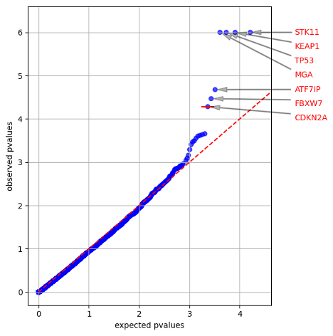
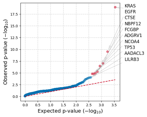
Both figures show the observed p-values for each gene (y-axis) plotted against the expected p-value predicted by the null hypothesis (x-axis), therefore a large deviation from the dashed line towards the y-axis is indicative of greater mutation functional impact (oncodriveFML) or mutation clustering (oncodriveCLUSTL) than expected by chance for a gene. Genes with a significant q-value are labeled in each plot.
Both algorithms also generate .tsv files containing the p- and q-values for all tested genes, plus other miscellaneous statistics such as counts of mutations per gene and individual cluster statistics for OncodriveCLUSTL (descriptions for output: OncodriveFML,OncodriveCLUSTL).
Many significant driver genes identified do not overlap in these two sample sets. To explain why these results are so different, take a look at OncodriveCLUSTL’s mutation clusters for KRAS and TP53, generated using a cohort of 1000+ samples:


Strongly clustered mutation patterns like KRAS will be strongly selected by OncodriveCLUSTL whereas genes like TP53 may be missed due to weak clustering. This further illustrates why synthesizing the results from many algorithms with different strengths and weaknesses can produce a better result than relying on only one.
When your jobs completes (~5 minutes), you should get the following quantile plots from analyzing only chr17:


dNdScv
Overview
dNdScv is an R package that contains a group of maximum-likelihood dN/dS methods for quantifying selection at the gene level. More specifically, dN/dS ratio refers to the normalized ratio of non-synonymous to synonymous mutations (dN/dS). Non-synonymous mutations are a change in the coding sequence which cause a change in an amino acid of a protein sequence, while synonymous mutations do not change the amino acid in the protein sequence. Genes which experience non-synonymous mutations significantly more often than synonymous mutations are expected to be under selection for gain/loss of function mutations, as expected for cancer drivers.
- dN/dS ratio > 1 implies selection for gain/loss/change of function mutations, or ‘positive’ selection
- dN/dS ratio < 1 implies purifying, or ‘negative’, selection
- dN/dS ratio = 1 indicates no selection, or ‘neutrality’
The dN/dS ratio was originally developed as a method to detect gene-level species evolution in the context of phylogenetics. The dNdScv method adapts dN/dS for improved performance in somatic contexts for whole-exome, whole-genome, and targeted sequencing studies. dNdScv uses trinucleotide context-dependent substitution models to avoid common mutation biases affecting dN/dS and exploits global information (variation of the mutation rate across genes, exploiting epigenomic covariates) to estimate the background mutation rate of each gene.
Use the following links for additional information regarding the dNdScv package:
- Publication for dNdScv: https://doi.org/10.1016/j.cell.2017.09.042
- GitHub page for dNdScv: https://github.com/im3sanger/dndscv
Download session folder
First we will download the folder we have created for this session. This zipped folder, session8_dndscv.zip, can be downloaded here.
This folder should download directly to your /Downloads folder. After it downloads, unzip the folder as you normally would on your machine.
This folder includes several files:
- the mutational data we will be using today from a subset of the Sherlock-Lung Study
- the R script with all of the commands you will find throughout this part of the practical session
- covariate file.
The covariate file and a genome reference file, which we will download in R, are necessary to run dNdScv.
Open the file, dndscv_session8_practice_FINAL.R. This should open in RStudio.
Install and load dNdScv package in R
1. There are some additional packages we will need today to run the R code. Run the following commands below to install these packages if they are not already installed:
packages_req <- c('tidyverse','devtools','scales','hrbrthemes')
pkg_check_fcn <-lapply(packages_req,function(x){
  if(!(x %in% installed.packages())){
    install.packages(x, dependencies = TRUE, repos=structure(c(CRAN="http://cloud.r-project.org/")))
    library(x, character.only = TRUE)
  }else{
    library(x, character.only = TRUE)
  }
})
The code above checks to see if the necessary packages are installed, and installs them if they are not. Then, those packages are loaded into the environment.
2. If you haven’t done so already, you will need to install the dndscv package in R. Use the following commands to do this:
install_github("im3sanger/dndscv")
After you install dndscv, load the package using the library() command:
library(dndscv)
Load the data into R
3. Run getwd() to make sure that the current working directory is the path to the session8_dndscv folder:
getwd()
### Mac:
[1] "/Users/[username]/Downloads/session8_dndscv"

### Windows:
[1] "C:/Users/[username]/Downloads/session8_dndscv"
4. **If the working directory is not the session8_dndscv directory, use the setwd() command to set this directory as the working directory.
-
Mac:
setwd("/Users/[username]/Downloads/session8_dndscv") -
Windows:
setwd("C:/Users/[username]/Downloads/session8_dndscv")
Then run getwd() again to make sure the working directory is now correct:
getwd()
### Mac:
[1] "/Users/[username]/Downloads/session8_dndscv"

### Windows:
[1] "C:/Users/[username]/Downloads/session8_dndscv"
The data we will be using to run dNdScv is the same data used to run OncodriveFML and OncodriveCLUSTL- mutational data from 200 samples from the Sherlock-Lung project.
To load the mutation data file, we will need to use the path to the file so it can be loaded into R. Since we are already in the directory where the file is stored, we only need to use the name of the file.
5. Use the command below to load the data file:
sherlock_mdata <- read_delim("sherlock_only_mutations_top200.txt.gz")
This file should take 30 seconds or less to load. When it is finished loading, check your Environment tab to make sure that you now see the sherlock_mdata object in your environment.
Explore and Prepare Data
6. You could also check the dimensions of the data you just loaded, using the dim() command:
dim(sherlock_mdata)
[1] 13076340 5
You should see that you have 13076340 rows of mutation data, and 5 columns.
7. To get a sense of what the data looks like, use the head() command to print the first several lines to the console:
head(sherlock_mdata)
# A tibble: 6 × 5
  Tumor_Sample_Barcode   Chr   Start Ref         Alt
  <chr>                <dbl>   <dbl> <chr>       <chr>
1 NSLC-0005                1  666315 G           C
2 NSLC-0005                1  783512 G           C
3 NSLC-0005                1  784070 G           A
4 NSLC-0005                1  871285 G           T
5 NSLC-0005                1 1121013 AGGCTCGGTT… A
6 NSLC-0005                1 1308517 C           T
Here, we can see the first six lines of our data, with the columns Tumor_Sample_Barcode, Chr, Start, Ref, and Alt. In other words, these columns are the sample ID, the chromosome, the start position, reference allele, and alternative allele.
To run dNdScv, we need the columns in our data to match the required input column names for the tool. We need our columns to be the following: sampleID, chr, pos, ref, mut.
8. To change our columns in R, we can do the following:
colnames(sherlock_mdata) <- c('sampleID', 'chr','pos','ref','mut')
This changes our column names. To check that they were changed, we can run the colnames() command again:
colnames(sherlock_mdata)
[1] "sampleID" "chr" "pos" "ref" "mut"
And we see that your column names are correct.
9. We will now set another object, which we are calling dndsout, to NULL, so we can then store the output here.
dndsout <- NULL
10. We also need to load the covariate file, which can be found in the folder you originally downloaded at the beginning of this session. This data is used to aid in estimating the background mutation rate of each gene.
This file contains covariate data that was generated combining epigenomic data (from Roadmap Epigenomics) and whole-genome mutation density vectors (from the PCAWG consortium), collapsed into 20 principal components per gene.
load("covariates_hg19_hg38_epigenome_pcawg.rda")
This is loaded into your environment as an object named covs.
Note: It is important to be sure to use the correct covariate file depending on the genome build your data is based on. This newer covariate file is convenient as it can be used for both GRCh37/hg19 and GRCh38/hg38. However, this covariate file is only compatible with specific RefCDS objects, which are as follows:
- GRCh38: RefCDS_human_GRCh38_GencodeV18_recommended.rda
- Hg19: RefCDS_human_hg19_GencodeV18_newcovariates.rda
Since our data uses GRCh38, we will use the RefCDS object, RefCDS_human_GRCh38_GencodeV18_recommended.rda, along with the covariates_hg19_hg38_epigenome_pcawg.rda covariate file for the analysis.
This RefCDS object contains data and information for the coding sequence data for each gene included in the object. Download this file from the github dndscv_data repository:
download.file("https://github.com/im3sanger/dndscv_data/raw/master/data/RefCDS_human_GRCh38_GencodeV18_recommended.rda",
              destfile = "./RefCDS_human_GRCh38_GencodeV18_recommended.rda")
Additional Information: While not necessary, you can also load the genome reference file into the environment if you’d like.
load('RefCDS_human_GRCh38_GencodeV18_recommended.rda')
If you load this data, and then click on RefCDS in the R environment, you will see that there is a list of over 19,000 genes with sub-lists containing information for each gene. This reference will be used when we run dNdScv in the next step.
Run dndscv
11. To run dNdScv, we will set up a function call:
dndsout <- dndscv(mutations = sherlock_mdata, refdb = 'RefCDS_human_GRCh38_GencodeV18_recommended.rda',cv =covs)
In this run of dNdScv, we use the following parameters:
mutationsis set to our mutation datarefdbis set to a RefCDS object which we downloaded earliercvis set to the covariate data (covs) you loaded into the R environment
This will take about two and a half minutes to run. You will see updates printed to the console periodically, like the following:
[1] Loading the environment...
[2] Annotating the mutations...
Note: 1 samples excluded for exceeding the limit of mutations per sample (see the max_coding_muts_per_sample argument in dndscv). 199 samples left after filtering.
Note: 535 mutations removed for exceeding the limit of mutations per gene per sample (see the max_muts_per_gene_per_sample argument in dndscv)
11% ...
21% ...
32% ...
42% ...
53% ...
63% ...
74% ...
85% ...
95% ...
[3] Estimating global rates...
[4] Running dNdSloc...
[5] Running dNdScv...
Regression model for substitutions (theta = 6.58).
Regression model for indels (theta = 5.2)
Warning messages:
 1: In dndscv(mutations = sherlock_mdata, refdb = "RefCDS_human_GRCh38_GencodeV18_recommended.rda",  :
Mutations observed in contiguous sites within a sample. Please annotate or remove dinucleotide or complex substitutions for best results.
2: In dndscv(mutations = sherlock_mdata, refdb = "RefCDS_human_GRCh38_GencodeV18_recommended.rda",  :
Same mutations observed in different sampleIDs. Please verify that these are independent events and remove duplicates otherwise.
We have run dNdScv with mostly default parameters. This includes removing ultra-hypermutator samples and subsampling mutations when encountering too many mutations per gene in the same sample. These were designed to protect against loss of sensitivity from ultra-hypermutators and from clustered artifacts in the input mutation table, but there are occasions when the user will prefer to adjust these as they see fit.
The theta values for substitutions and indels, 6.58 and 5.2, respectively, denote that the dataset is clean- typically theta values for clean datasets of somatic mutations is greater than 1. If this were less than 1, it would indicate that the mutation rate varies too much across genes.
The function issues a warning that there are mutations observed in contiguous sites within a sample. For today’s purposes this can be ignored, but in another circumstance it could be beneficial to look into these complex substitutions more closely.
The function issues a second warning as it detects the same mutation in more than one sample, requesting the user to verify that the input table of mutations only contains independent mutation events. In this case, each sample corresponds to a different patient and so the warning can be safely ignored.
When dNdScv is finished running, you will see the dndsout object generated in the Environment tab. The dndsout object consists of a list of objects.
Explore dndscv results
First, we are going to extract sel_cv, which includes the results of neutrality tests at the gene level via the dNdScv method.
12. We use the following command to extract sel_cv from the dndsout object:
sel_cv <- dndsout$sel_cv
We can view the data frame that we have extracted by using the following command, or simply click on the sel_cv data object found under the Environment tab:
sel_cv %>% View()
This data frames consists of 20 columns, which include include the following, and are with respect to a specific gene:
- Columns that start with ‘n’ are those containing a count of mutation type - synonymous (n_syn), missense (n_mis), nonsense (n_non), essential splice site (n_spl), indels (n_ind)
- Columns that start with ‘w’ are maximum-likelihood estimates of dN/dS ratios for a given gene for different type of mutations - missense (wmis), nonsense (wnon), essential splice site mutations (wspl) and indels (wind)
- Columns that start with ‘p’ are p-values - missense (pmis_cv), truncating (ptrunc_cv), all substitutions (pallsubs_cv), indels (pind_cv), all mutation types (pglobal_cv)
- Columns that start with ‘q’ are q-values - missense (qmis_cv), truncating (qtrunc_cv), all substitutions (qallsubs_cv), indels (qind_cv), all mutation types (qglobal_cv)
dN/dS ratios of significant cancer genes (columns that start with ‘w’) are typically extremely high, often >10 or even >100. This contains information about the fraction of mutations observed in a gene that are genuine drivers under positive selection. For example, for a highly significant gene, a dN/dS of 10 indicates that there are 10 times more non-synonymous mutations in the gene than neutrally expected (Greenman et al, 2006; Martincorena et al, 2017).
In our data output, we can see that the columns beginning with ‘w’, the estimates of dN/dS ratios, are very high for some of the genes, including, but not limited to, TP53 and KEAP1, KRAS.
13. If we filter our sel_cv dataframe for only the three genes noted above, TP53, KEAP1, and KRAS, we can see that the values for these different estimates vary across the different mutation types:
dnds_wvals <- sel_cv %>% filter(gene_name%in% c('TP53','KEAP1','KRAS')) %>% select(gene_name, starts_with('w'))
We can view the data frame that we have extracted by using the following command, or simply click on the sel_cv data object found under the Environment tab:
dnds_wvals %>% View()
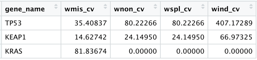
Here we can see that the TP53 has dN/dS ratio estimates that are high across all mutation types. In contrast, KRAS has a high estimate with regard to the missense mutation type. Overall, these higher values denote that a large proportion of mutations in these genes are genuine drivers.
14. Now, we will look into the q-values included in our results. The smaller the q-value, the less of a chance that the result is a false positive. We have several different q-values available in our result, as highlighted above. these include:
For our purposes today, let’s briefly look at those genes whose qglobal_cv value (which considers all mutation types) is less than 0.1. This q-value cutoff can differ depending on your type of analysis or what you are interested in investigating.
signif_genes = sel_cv[sel_cv$qglobal_cv<0.1, c("gene_name","qglobal_cv")]
If we look at the data frame, we can see that 18 genes meet this filtering criteria of having a q-value that is less than 0.1.
15. We can also explore additional data included in the dndscv output. Another result of the dndscv function is annotmuts, an annotated table of coding mutations. If we look at just the first several lines of the annotmuts table, we can see a variety of information about the mutations, including what samples they are from, coordinate information, codon information, amino acid change information, and gene information.
head(dndsout$annotmuts)
  sampleID   chr      pos   ref   mut   gene    strand
  <chr>     <chr>    <dbl> <chr> <chr> <chr>    <dbl>
1 NSLC-0005 1      6475486 C     G     PLEKHG5     -1
2 NSLC-0005 1     10337084 C     T     KIF1B        1
3 NSLC-0005 1     11022554 C     T     TARDBP       1
4 NSLC-0005 1     11649793 G     C     FBXO2       -1
5 NSLC-0005 1     16134505 G     C     EPHA2       -1
6 NSLC-0005 1     21978410 G     A     CELA3B       1
16. Using the annotated mutation data, we can calculate mutation frequency of specific genes to see in what proportion of samples a gene is mutated in our sample set. See the code below.
Get the sample size by using n_distinct() to count the number of unique sampleIDs:
sizedata <- n_distinct(sherlock_mdata$sampleID) - 1 # number of samples - 1
We subtract one from this total because one of the samples was removed due to exceeding the maximum coding mutation count per sample. We know to subtract one because of this in the dndscv function output printed in the console:
Note: 1 samples excluded for exceeding the limit of mutations per sample (see the max_coding_muts_per_sample argument in dndscv). 199 samples left after filtering.
As stated before, we ran dNdScv with mostly default parameters. One of these defaults removes ultra-hypermutator samples. This parameter was designed to protect against loss of sensitivity (i.e. potential bias) due to ultra-hypermutators, but can also be adjusted depending on the analysis.
Create a mutation frequency table. Note that for our purposes today we will focus on the 18 genes with a qglobal_cv value of <0.1:
freqdata <- dndsout$annotmuts %>%
  filter(gene %in% signif_genes$gene_name) %>%
  filter(impact!="Synonymous") %>%
  count(sampleID,gene) %>%
  select(-n) %>%
  count(gene) %>%
  arrange(desc(n)) %>%
  mutate(Freq=100*n/sizedata)
If we look at just the first few lines in freqdata, we can see that the data frame consists of the gene, the number of samples with at least one mutation in the gene, and the frequency, or the percentage of samples in our sample set that had a mutation in the gene.
17. Now, we can take the frequency data and join this with the sel_cv data for the 18 significant genes (based on the qglobal_cv value) and generate a plot that looks at the relationship between mutation frequency and the (-log10 of the) qvalue.
p <- sel_cv %>% filter(gene_name %in% signif_genes$gene_name) %>%
  left_join(freqdata,by=c('gene_name'='gene')) %>%
  mutate(gene_name=factor(gene_name),gene_name=fct_reorder(gene_name,qglobal_cv)) %>%
  pivot_longer(cols = "qglobal_cv") %>%
  mutate(value=if_else(value==0,1e-16,value)) %>%
  ggplot(aes(Freq,-log10(value),fill=-log10(value)))+
  geom_point(pch=21,size=4,col="white",stroke=0.5)+
  ggrepel::geom_text_repel(aes(label=gene_name),size=3.5)+
  ggtitle("Mutational frequency vs. qglobal values") +
  geom_hline(yintercept = c(1,16),col=c('red','purple'),linetype=2,alpha=0.5) +
  scale_x_continuous(breaks = breaks_pretty())+
  scale_y_continuous(breaks = breaks_pretty())+
  labs(x='Mutational Frequency (%)',y='-log10(qvalue)')+
  theme_ipsum(axis_title_just = 'm',axis_title_size = 14,grid = 'XYx',ticks = TRUE,axis   = FALSE)+
  theme(legend.position = 'none') + coord_cartesian(clip = "off")
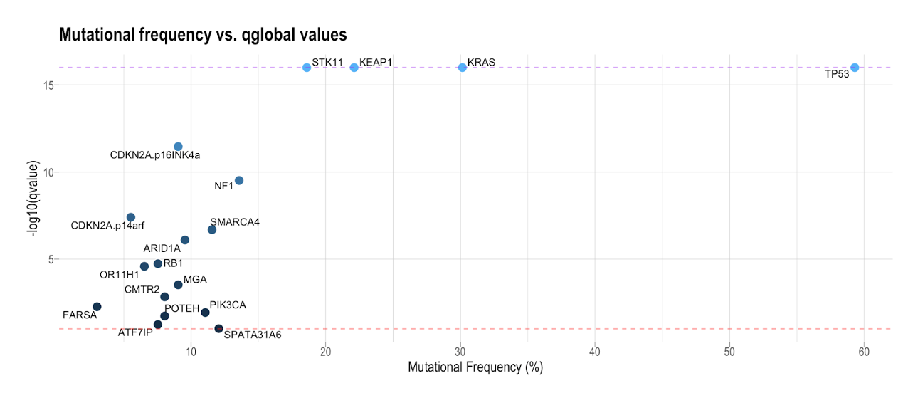
The coloration of the dots is based on the -log10(qvalue). We can see that there is a cluster of genes with a low mutational frequency and a slightly larger q-value in the bottom left of each plot. Those in the top right of the plot have a high mutational frequency and a small q-value (i.e. highly significant). The two horizontal lines across the plot are the cutoffs for:
- genes whose qvalue was 0 (purple line)
- genes whose qvalue just met the less than 0.1 criteria (red line).
We see several common drivers at a lower frequency in these samples compared to other common drivers at a higher frequency, such as TP53 and KRAS. Statistically significant, low-frequency mutated genes may be false positives or may represent rare cancer drivers in a specific cancer type (e.g. ARID1A in this specific case). Some cancers, e.g. prostate cancer, (https://www.ncbi.nlm.nih.gov/pmc/articles/PMC6107367/), have rare driver mutations in many genes. Looking at both mutational frequency and q-value is just one way of exploring the data that may help you narrow your focus for further analysis.
Based on the plots generated above, and our exploration of the different dN/dS ratios and the corresponding q-values, it could be concluded that these 18 genes are candidate cancer driver genes in our sample set. However, this sort of conclusion heavily depends on what you are interested in e.g. q-values cutoff, consideration of mutational frequency in determining drivers, etc.
OncodriveFML, OncodriveCLUSTL, and dNdScv Comparison
Now that we have run OncodriveFML, OncodriveCLUSTL, and dNdScv, let’s compare their results. In the table below, we have noted which genes were identified as drivers and by which algorithms. We have highlighted genes identified by at least 2 algorithms, which are the least likely to be false positives (though of course you may note that this excludes some known cancer drivers which were detected by only one algorithm, most notably EGFR).
| Gene | dNdScv | OncoFML | OncoCLUSTL |
|---|---|---|---|
| TP53 | TRUE | TRUE | TRUE |
| KEAP1 | TRUE | TRUE | |
| STK11 | TRUE | TRUE | |
| CDKN2A | TRUE | TRUE | |
| MGA | TRUE | TRUE | |
| ATF7IP | TRUE | TRUE | |
| KRAS | TRUE | TRUE | |
| NF1 | TRUE | ||
| SMARCA4 | TRUE | ||
| ARID1A | TRUE | ||
| RB1 | TRUE | ||
| OR11H1 | TRUE | ||
| CMTR2 | TRUE | ||
| FARSA | TRUE | ||
| PIK3CA | TRUE | ||
| POTEH | TRUE | ||
| SPATA31A6 | TRUE | ||
| FBXW7 | TRUE | ||
| EGFR | TRUE | ||
| CTSE | TRUE | ||
| NBF12 | TRUE | ||
| FCGBP | TRUE | ||
| ADGRV1 | TRUE | ||
| NCOA4 | TRUE | ||
| AADACL3 | TRUE | ||
| LILRB3 | TRUE |
This is a common method for manually combining the results from several algorithms, commonly referred to as “voting”, and of course the number of votes needed would change depending on your analysis and how many algorithms you used.
Even better than manually combining results is using an automated statistical or machine learning method such as IntoGen, which is a carefully developed pipeline for combining results from 7 cancer driver gene algorithms, including the three we practiced with today.
Note: As of this writing, IntoGen is in the process of being installed on Biowulf and will be available soon.
Cancer Genome Interpreter (CGI)
Overview
CGI is a platform that systematizes the interpretation of cancer genomes, the main hallmark of which is the streamlining and automatization of the whole process. There are two main components of the CGI platform, including:
1. Identification of all known and likely tumorigenic genomic alterations (point mutations, small insertions/deletions, copy number alterations and/or gene fusions) of a tumor, including the assessment of variants of unknown significance.
2. Annotation of all variants of the tumor that constitute biomarkers of drug response organized using different levels of clinical evidence.
The publication for the first release of CGI can be found here: https://genomemedicine.biomedcentral.com/articles/10.1186/s13073-018-0531-8
Researchers and clinicians can utilize a tool like CGI to support cancer research projects and guide preclinical experiments, as well as an additional resource when selecting the best treatment option for a patient.
The following is a two minute overview of what Cancer Genome Interpreter is and why it is useful. It is a great way to begin to understand CGI:
The following link will take you to the homepage of Cancer Genome Interpreter. Here you will find the video mentioned above, as well as an additional video about a method used in CGI, called BoostDM: https://www.cancergenomeinterpreter.org/home.
CGI Framework
The main steps of the CGI framework include those listed below:
- CGI takes genomic alterations as input and automatically recognizes the format, remaps variants as necessary, and standardizes annotation.
- Identifies likely driver alterations in cancer driver genes in the tumor type (BoostDM and OncoDriveMut), and annotates mutations in the tumor that are known to be tumorigenic.
- Identifies alterations that constitute biomarkers of response to anti-cancer drugs.

Link to image: https://www.cancergenomeinterpreter.org/faq#q02
Below is a figure depicting how the driver events are identified, through the use of either BoostDM or OncoDriveMut:

First, CGI determines if the gene is a driver gene. If so, likely driver alterations in the gene are then identified by one of the two approaches used: BoostDM or OncoDriveMut. Indels are further analyzed by OncoDriveMut, whereas point mutations are further analyzed by BoostDM, if there is a gene-specific BoostDM model available. Otherwise, OncoDriveMut is used. If you are interested, here is a link to a two minute video highlighting the basics of BoostDM: https://www.youtube.com/watch?v=1Nq_rm_yudk&t=8s
Identifying Driver Genes using CGI
There are a series of tabs across the top of the CGI homepage. Feel free to browse some of the tabs on your own.

In addition to these tabs, you can also access all of the different mutation, gene, and biomarker data that are utilized in CGI using the following links:
Genes: https://www.cancergenomeinterpreter.org/genes
Mutations: https://www.cancergenomeinterpreter.org/mutations
Biomarkers: https://www.cancergenomeinterpreter.org/biomarkers
Note: The Cancer Bioactivities database is no longer supported in CGI.
1. To use CGI, go to the Analysis tab, or click the following link: https://www.cancergenomeinterpreter.org/analysis

Below is the CGI Analysis page. This is where we will upload the mutation data we wish to analyze, and select the cancer type and reference genome.

You can view several CGI examples and their output by clicking View CGI example results in the top right corner. These examples are helpful to see what types of data have been run, and what the results of CGI look like.
Also notice that you can insert a mutation per line in various formats, as you can see in the Alterations box. For our purposes today, we will be uploading a mutation file.
2. Today’s example will only use one sample from the Sherlock-Lung project, due to time restraints. Click here to download the file with mutation data for one sample, NSLC-0005.
3. Decompress the file as you normally would on your machine.
4. To upload a file, click the Add file + button in the Alterations table. Navigate to the folder housing the NSLC-0005_example.txt file and select the file.
5. Now we can set up our other inputs for the interpreter. First, we will select Solid Tumors → Torax → Lung → Non-small cell lung. Make sure the NSCLC option is selected with a pink rectangle. See below:

6. Make sure the reference genome is set to hg38.
7. Click Run.
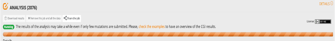
8. This will take just under about 18 minutes to run. While your job is running, you will see the following at the top of the screen:
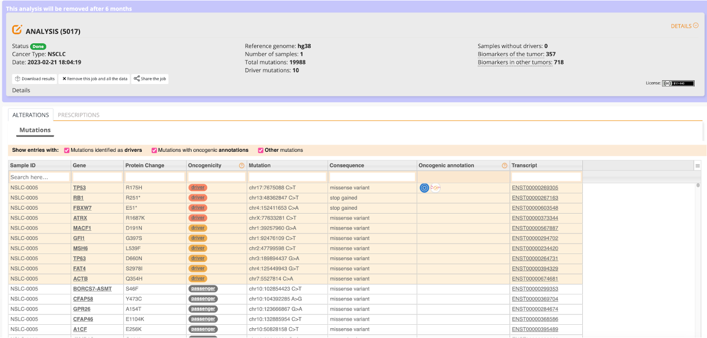
When the job completes, you will see a screen that looks something like this:
9. While you are waiting for this job to complete, we will take a look at the results using the following link: https://www.cancergenomeinterpreter.org/analysis?id=3ff8aca92ef238385e58.
At the top of the screen in the gray box we can see the details of our job submission. We can see, for example, that we ran one sample (shown in sample ID column of the table, NSLC-0005) and there were a total of almost 20,000 mutations in just this one sample, with 10 driver mutations.
Completion of the job automatically takes you to the Alterations table. In this table, we see all of the different results from the mutation analysis, including but not limited to: gene name, mutation, protein change, oncogenicity, and consequence of the mutation in a given gene. Several of these columns also link to other pages. For example, the Oncogenic annotation for EGFR will take you to OncoKB for additional information.
We will use this table to determine what genes are potential drivers in this sample.
By hovering over the value in the Oncogenicity column, we can see which approach identified the specific gene and the corresponding mutation as a driver (i.e. either BoostDM or OncoDriveMut).
In the case of this one sample, there were four drivers identified by the BoostDM approach, and six drivers identified by the OncodriveMUT approach. The remainder of the results are considered passengers. For a quick summary, below is a table of all of the driver genes identified in this sample and their corresponding driver mutations:
| Gene | Protein Change | Mutation |
|---|---|---|
| TP53 | R175H | chr17:7675088 C>T |
| RB1 | R251* | chr13:48362847 C>T |
| FBXW7 | E51* | chr4:152411653 C>A |
| ATRX | R1687K | chrX:77633281 C>T |
| MACF1 | D191N | chr1:39257960 G>A |
| GFI1 | G397S | chr1:92476109 C>T |
| MSH6 | L539F | chr2:47799598 C>T |
| TP63 | D660N | chr3:189894437 G>A |
| FAT4 | S2978I | chr4:125449943 G>T |
| ACTNB | Q354H | chr7:5527814 C>A |
The second table you will find in the output from CGI is the Prescriptions table. This table contains annotations of all variants of the tumor that constitute biomarkers of drug response, and are organized using different levels of clinical evidence. These levels of evidence range from A-D, with A being the highest level of evidence, guidelines of FDA approved drugs, to D, pre-clinical studies.
Level of Evidence Description:
| Level of Evidence | Description |
|---|---|
| A | corresponds to biomarkers used in professional guidelines of FDA approved drugs |
| B | groups biomarkers observed in clinical trials |
| C | corresponds to biomarkers identified from small group studies or case studies |
| D | biomarkers have been identified in pre-clinical studies |
There are several different pieces of information displayed for the mutations found in the sample(s) uploaded and the biomarkers these mutations matched, including:
- Drugs the biomarker is associated with
- Disease and tumor type
- Response to a drug
- Level of evidence
- Source database for where the information for a given mutation-biomarker match comes from
For example, if we search in the Prescription table for the first driver in our Alterations table, TP53, and focus on the R175H amino acid change, we see that there are two different biomarker matches.
The first biomarker, TP53 (R248Q, R175H), corresponds to response to HSP90 inhibitors in any cancer type. However, the level of evidence is low, at level D, meaning that this has only been identified in pre-clinical studies.
The second biomarker, TP53 oncogenic mutation, corresponds to response to the drug combination of Docetaxel and Selumetinib in non-small cell lung cancer. However, as with the first biomarker, this is also only with a ‘D’ level of evidence. In contrast, Docetaxel on its own corresponds to the resistance in non-small cell lung cancer.
From just this one example, it can be seen that CGI can serve as a great tool in analyzing alterations that constitute biomarkers of response to anti-cancer drugs, furthering knowledge and understanding of alterations and cancer therapies.
Additional Information: You can also choose to download the results by clicking the Download results button in the top left. This will download a zip folder to the Downloads folder on your computer. If you unzip this folder, you will see that there are three files included:
- drug_prescription.tsv- prescriptions table you see in the CGI result page, give or take a few columns. Includes all biomarkers identified, regardless of tumor type.
- input01.tsv- the file uploaded as input for the job submission
- mutation_analysis.tsv- alterations table you see in the CGI result page, give or take a few columns