Presenters: Jian Sang, Azhar Khandekar

Introduction

This session aims to provide a comprehensive guide to identify somatic copy number alterations in cancer genomic studies. We will use the FACET and ASCAT algorithms, and whole genome sequencing data from one tumor and normal pair to demonstrate the key steps in somatic copy number alterations calling. Then we will introduce how to identify significant SCNA regions using GISTIC2. Finally, we will show you how to perform somatic copy number alteration signatures analysis with SigProfilerMatrixGenerator and SigProfilerExtractor.

Log into Biowulf and set up interactive session

Before we begin, please login to Biowulf and request an interactive session:

For a reminder on how to log-in to Biowulf, we refer you to this Biowulf HPC guide.

In short:

• Windows users: use PuTTy
• Mac users: open your terminal and enter ssh biowulf.nih.gov followed by your password when prompted.

After you login to Biowulf, please request an interactive session with the following command:

sinteractive --gres=lscratch:4 --mem=10g --cpus-per-task=4 --time=02:00:00

The sinteractive command is used to start an interactive session on a Slurm cluster. The –gres=lscratch:4 option specifies that the job should be allocated 4 Gb of local scratch space, which is a type of temporary storage that is typically used for high-speed I/O or as a workspace for computations. The –mem=10g option specifies that the job should be allocated 10 GB of memory. The –cpus-per-task=4 option specifies that the job should be allocated 4 CPU cores. The –time=02:00:00 option specifies that the job should be allowed to run for a maximum of 2 hours.

To access the output results, we suggest mounting your Biowulf working directory on your local computer. If you need help with this, you can refer to the biowulf helping document (Locally Mounting HPC System Directories).

Identification of somatic copy number alterations using FACETS

FACETS is an Allele-Specific Copy Number (ASCN) analysis tool with a broad application to whole genome, whole-exome, as well as targeted panel sequencing platforms. It can provide an integrated SCNA calling pipeline that includes sequencing data processing, segmentation, purity & ploidy estimation, and visualisation. According to the latest statistics from google scholar, this tool has been cited ~700 times, since its first publication in 2016.

Once your interactive session is ready:

1. Change the current working directory to /data/$USER/, where $USER is the current user’s username.

cd /data/$USER/

2. Create a new directory called practical_session_7 in the current working directory.

mkdir practical_session_7

3. Change the current working directory to practical_session_7.

cd practical_session_7

4. Create a dir “Facets” for running this tool

mkdir Facets
cd Facets

5. Copy the file session_7_sbatch_facets.sh to the current working directory.

cp /data/classes/DCEG_Somatic_Workshop/Practical_session_7/facets_scripts/Session_7_1_facets_sbatch.sh .

6. Submit the file Session_7_sbatch_facets.sh to a workload manager (e.g., SLURM) using the sbatch command.

sbatch --cpus-per-task=2 --mem=40g --time=3:00:00 Session_7_1_facets_sbatch.sh

Note: the –cpus-per-task, –mem, and –time flags are options that specify the number of CPU cores, amount of memory, and maximum runtime for the job, respectively.

You can check the job running status using sjobs or squeue -u $USER.

7. The jobs may run for ~3 hours depending on the power of your assigned CPU. To save your time, please copy the result files from the expected result folders in your biowulf directory:

cp -r /data/classes/DCEG_Somatic_Workshop/Practical_session_7/Expect_result/FACETS_Output_Expected/ .

After mounting the HPC drive, users can check the expected result folder in their local system.

8. FACETS supports two kinds of formats as input:

Option 1: BAM files

Absolute path of a bam file from tumour sample

Absolute path of a bam file from normal sample

Option 2: Pileup files as input

The pileup is a comma separated file recording read counts of the reference allele and alternate allele at selected SNPs. This file must have the following columns (order of columns is not important, additional columns are ignored):

• Chromosome: Chromosome of the SNP or marker
• Position: Position of the SNP
• File1R: Read depth supporting the REF allele in normal sample
• File1A: Read depth supporting the ALT allele in normal sample
• File2R: Read depth supporting the REF allele in tumour sample
• File2A: Read depth supporting the ALT allele in tumour sample

9. Have a closer look at our sbatch script:

vim /data/$USER/practical_session_7/Facets/Session_7_1_facets_sbatch.sh

#!/bin/bash

#SBATCH -o Session_7_sbatch_1_facets.out
#SBATCH -e Session_7_sbatch_1_facets.err


### 001 packages need to be loaded
module load python/3.9
module load samtools/1.6
module load R

### 002 define facets_script, input and output
Input_Dir=/data/classes/DCEG_Somatic_Workshop/Practical_session_7/facets_scripts/InputDir
Output_Dir=`pwd`/output

facets_py_path=/data/classes/DCEG_Somatic_Workshop/Practical_session_7/facets_scripts/Session_7_1_FACETS.py

python $facets_py_path -i $Input_Dir -o $Output_Dir



# sbatch --cpus-per-task=2 --mem=40g --time=6:00:00 Session_7_1_facets_sbatch.sh

In this sbatch script, we define basic parameters like input and output for running facets program and submit it at biowulf.

• Line 1 is the header of this script, to tell biowulf the script should be interpreted by bash.
• Line 3 and Line 4 is used to produce log file to summarise output and error
• Line 8 to Line 10 is used to load basic environments required by facets.
• Line 13 and Line 14 is used to define the absolute path of input and output Directories
• Line 16 is used to define the absolute path of python program to run facets

10. Have a closer look at our Major pipeline to run facets:

vim /data/classes/DCEG_Somatic_Workshop/Practical_session_7/facets_scripts/Session_7_1_FACETS.py

Step 1: Define Necessary Parameters, e.g., Subject_ID, Barcode for Tumor sample and Normal sample. The absolute path of SNP_Pileup program, facets program and VCF file which select common SNPs for further segmentation.

#!/usr/bin/python
import re,os
import argparse


####### 001 Define_Basic_Parameters()
#Input_Dir = "/data/classes/DCEG_Somatic_Workshop/Practical_session_7/facets_scripts/InputDir"

Subject_ID = "Test"
bam_normal_Barcode = "Test_Normal"
bam_tumour_Barcode = "Test_Tumor"


SNP_Pileup_Bin = "/data/classes/DCEG_Somatic_Workshop/Practical_session_7/facets_scripts/facets-master/inst/extcode/snp-pileup"
run_facets_Bin = "/data/classes/DCEG_Somatic_Workshop/Practical_session_7/facets_scripts/run_facets.R"

vcf = "/data/classes/DCEG_Somatic_Workshop/Practical_session_7/facets_scripts/00-common_all.vcf.gz"

#Output_Dir = "/data/sangj2/z-19-temp/Practical_session_7/0-FACETS/FACETS_Output"

####### 000-1 Extract Parser
def Parser():
	parser = argparse.ArgumentParser()

	parser.add_argument('-i', '--Input_Dir', required=True, type=str, help="Input_Dir")
	parser.add_argument('-o', '--Output_Dir', required=True, type=str, help="Output_Dir")

	args = parser.parse_args()
	return args.Input_Dir, args.Output_Dir

Step 2: Run snppileup. (Including absolute path of Snp_Pileup, common_VCF, Input Bam files and output_Path of Snp_Pileup)

####### 003 Run_snppileup()
def Run_snppileup(Input_Dir, Output_Dir):
	Note_1 = "\n####### Running SNP_PileUP... \n\n"
	print(Note_1)

	bam_normal_Path = "%s/Normal.cram" % Input_Dir
	bam_tumour_Path = "%s/Tumor.cram" % Input_Dir

	snppileup_Output_Path = "%s/%s.snp.csv.gz" % (Output_Dir, Subject_ID)
	#cmd = "%s -g -q15 -Q20 -P100 -r25,0 %s %s %s %s" % (SNP_Pileup_Bin, vcf, snppileup_Output_Path, bam_normal_Path, bam_tumour_Path)
	cmd = "%s -g -q15 -Q20 -r20,30 %s %s %s %s" % (SNP_Pileup_Bin, vcf, snppileup_Output_Path, bam_normal_Path, bam_tumour_Path)

	print(cmd)
	os.system(cmd)

	####### Running Time:  2 cpus, 4 Gb, 1.5 hour

Step 3: Run facets. (Including absolute path of facets, Snp_Pileup results, subject ID, Output directory)

####### 004 Run_facets()
def Run_facets(Output_Dir):

	Note_2 = "\n####### Running Facets... \n\n"
	print(Note_2)

	snppileup_Output_Path = "%s/%s.snp.csv.gz" % (Output_Dir, Subject_ID)

	cmd = "Rscript %s %s %s %s" % (run_facets_Bin, snppileup_Output_Path, Subject_ID, Output_Dir)

	print(cmd)
	os.system(cmd)

	####### Running Time:  2 cpus, 40 Gb, 15 minutes

Check FACETS output

11. Check our expected output:

tree /data/$USER/practical_session_7/Facets/FACETS_Output_Expected/

├── Test_facets.pdf
├── Test_purity_ploidy_facets.txt
├── Test_segments_facets.txt
└── Test.snp.csv.gz

0 directories, 4 files

*_segments_facets.txt is the major output file with 14 columns (https://github.com/dariober/cnv_facets)

less /data/$USER/practical_session_7/Facets/FACETS_Output_Expected/Test_purity_ploidy_facets.txt

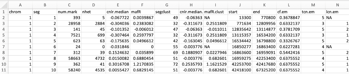
• chrom: Chromosome of the Segmentation
• seg: Segmentation ID
• num.mark: Number of SNPs in the segment
• NHET: Number of markers of heterozygous SNPs
• cnlr.median: Median log-ratio (logR) of each segment.
• mafR: Log-odds-ratio (logOR) of each segment.
• segclust: Segment cluster to which the segment belongs
• cnlr.median.clust Median log-ratio (logR) of the segment cluster.
• mafR.clust: Log-odds-ratio (logOR) summary for the segment cluster.
• start: start position of each segment
• end: end position of each segment
• cf.em: Fraction of DNA associated with the aberrant genotype.
• tcn.em: Total copy number.
• lcn.em: Minor copy number.

[sample name]_purity_ploidy_facets.txt includes the purity and ploidy of the tumor sample, estimated by the FACETS

sample  purity  ploidy
Test    0.640416509675053       4.02317905682627

Session_facets.pdf: Summary of identified SCNAs profile across the whole genome of the tumor sample.

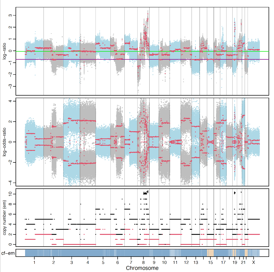
​​This is a general result as an example. In practice, you need to do a few steps for optimization of several parameters, to reduce background noise and remove segmentation with very small size (https://github.com/mskcc/facets).

Identification of somatic copy number alterations using ASCAT

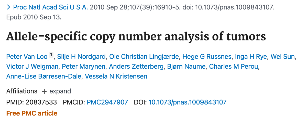
ASCAT is another famous tool for Allele-Specific Copy Number (ASCN) analysis. It can identify the ASCN from tumor samples, estimating and adjusting for both tumor ploidy and purity. The ASCAT tool was originally developed based on SNP array data. Now, the developers have updated it to support next generation sequencing data (ASCAT_NGS). According to the latest statistics from google scholar, ASCAT has been cited ~1100 times, since its first publication in 2010.

Note: The current version of ASCAT_NGS only supports whole genome sequencing data, if you would like to try other data type like exon sequencing, you need to contact their developers at (https://www.crick.ac.uk/research/labs/peter-van-loo/software) for help.

12. Change the current working directory to practical_session_7, where $USER is the current user’s username.

cd /data/$USER/practical_session_7/

13. Create a dir “ASCAT_NGS” for running this tool

mkdir ASCAT_NGS
cd ASCAT_NGS

14. Copy the file session_7_sbatch_ASCAT_NGS.sh to the current working directory.

cp /data/classes/DCEG_Somatic_Workshop/Practical_session_7/ASCAT_NGS/Session_7_2_ASCAT_NGS_sbatch.sh .

15. Submit the file session_7_sbatch_ASCAT_NGS.sh to a workload manager (e.g., SLURM) using the sbatch command. With 30 Cores CUP and 40g memory, the job can usually be finished within 1 hour.

sbatch --cpus-per-task=30 --mem=40g --time=2:27:27 Session_7_2_ASCAT_NGS_sbatch.sh

You can always check the status of the jobs by entering squeue -u $USER or sjobs.

16. Required environment for running ASCAT:

The above environment of ASCAT has been set up in Biowulf! Load this environment with the following code before running ASCAT:

module load ascatngs

17. Required input file:

• Tumour bam or cram: aligned whole-genome sequencing for tumor sample
• Normal bam or cram: aligned whole-genome sequencing for normal sample
• Genome.fa: reference genome (with associated *.fai index file). This must be the reference used to map of the input data
• SnpGcCorrections.tsv: GC correction windows for each SNP position used for Segmentation and SCNA calling

18. Details of sbatch script:

vim /data/$USER/practical_session_7/ASCAT_NGS/Session_7_2_ASCAT_NGS_sbatch.sh

#!/bin/bash
#SBATCH -o sbatch_output.txt
#SBATCH -e sbatch_error.txt

module load ascatngs


Input_Dir=/data/classes/DCEG_Somatic_Workshop/Practical_session_7/facets_scripts/InputDir
Output_Dir=/data/$USER/practical_session_7/ASCAT_NGS/output

bam_normal_Path=$Input_Dir/NSLC-AKVX-NT1-A-1-1-D-A81L-36.cram
bam_tumour_Path=$Input_Dir/NSLC-AKVX-TTP1-A-1-1-D-A81L-36.cram



reference_hg38_Path=/fdb/igenomes/Homo_sapiens/NCBI/GRCh38/Sequence/WholeGenomeFasta/genome.fa
snpGcCorrections_Path=/data/classes/DCEG_Somatic_Workshop/Practical_session_7/ASCAT_NGS/reference/SnpGcCorrections.tsv


ascat.pl \
-outdir $Output_Dir \
-tumour $bam_tumour_Path \
-normal $bam_normal_Path \
-reference $reference_hg38_Path \
-snp_gc $snpGcCorrections_Path \
-gender XX \
-genderChr Y \
-protocol WGS \
-platform ILLUMINA \
-species Human \
-assembly GRCh38 \
-cpus 30 \
-noclean \
-nobigwig

• Line 1 is the header of this script, to tell biowulf it is generated in the bash program.
• Line 2 and Line 3 is used to produce log file to summarise output and error
• Line 5 is used to load ASCAT NGS as well as the required running environment
• Line 8 to Line 9 is used to define the absolute path of tumor and normal bam files.
• Line 14 and Line 15 is used to define the absolute path of reference file
• Line 18 to Line 32 is used to run the ascat program for identification of SCNA.

19. To explore the expected results while the job is running, copy the result files from the expected result folders in your biowulf directory:

cp -r /data/classes/DCEG_Somatic_Workshop/Practical_session_7/Expect_result/Expect_result_ASCAT_NGS .

After mounting the HPC drive, users can check the expected result folder in their local system.

Output:

tree /data/$USER/practical_session_7/ASCAT_NGS/Expect_result_ASCAT_NGS/

├── NSLC-AKVX-TTP1-A-1-1-D-A81L-36.ASCATprofile.png
├── NSLC-AKVX-TTP1-A-1-1-D-A81L-36.ASPCF.png
├── NSLC-AKVX-TTP1-A-1-1-D-A81L-36.copynumber.caveman.csv
├── NSLC-AKVX-TTP1-A-1-1-D-A81L-36.copynumber.caveman.vcf.gz
├── NSLC-AKVX-TTP1-A-1-1-D-A81L-36.copynumber.caveman.vcf.gz.tbi
├── NSLC-AKVX-TTP1-A-1-1-D-A81L-36.copynumber.txt.gz
├── NSLC-AKVX-TTP1-A-1-1-D-A81L-36.germline.png
├── NSLC-AKVX-TTP1-A-1-1-D-A81L-36.rawprofile.png
├── NSLC-AKVX-TTP1-A-1-1-D-A81L-36.samplestatistics.txt
├── NSLC-AKVX-TTP1-A-1-1-D-A81L-36.sunrise.png
└── NSLC-AKVX-TTP1-A-1-1-D-A81L-36.tumour.png

0 directories, 11 files

Explore ASCAT output

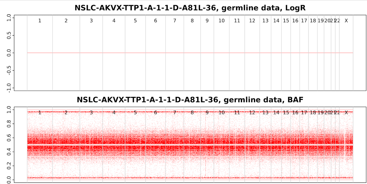
19-1 Germline Sample (NSLC-AKVX-TTP1-A-1-1-D-A81L-36.germline.png)

LogR and BAF plots from Germline sample. LogR points are around 0 and B allele frequency points are around 0.5. There are no obvious copy number changes from normal samples.

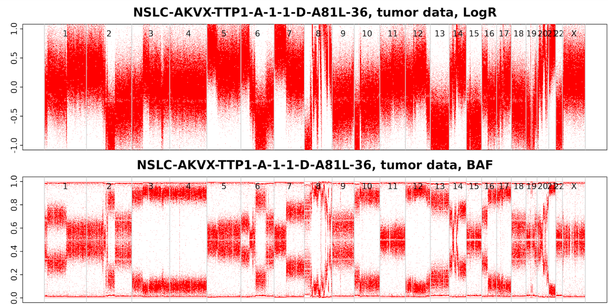
19-2 Tumor Sample (NSLC-AKVX-TTP1-A-1-1-D-A81L-36.tumour.png)

LogR and BAF plots from Tumor sample. Obviously, the tumor BAF plot and LogR plot are more variable than germline samples; a lot of clear segmentations can be observed across the tumor genome.

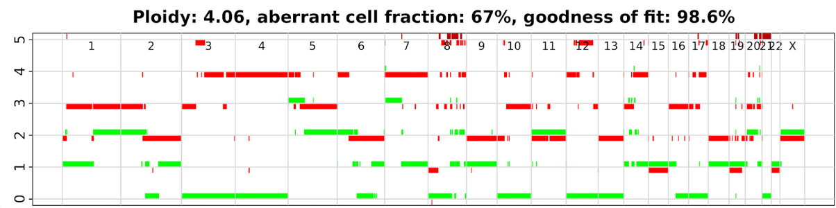
19-3 ASCAT Profile (NSLC-AKVX-TTP1-A-1-1-D-A81L-36.ASCATprofile.png)

Open NSLC-AKVX-TTP1-A-1-1-D-A81L-36.ASCATprofile.png. The ASCAT profile displays major and minor copy numbers (red/green), respectively. Major copy number refers to the greater copy number within two strands of the human genome. Minor copy number refers to the smaller copy number within two strands of the human genome.

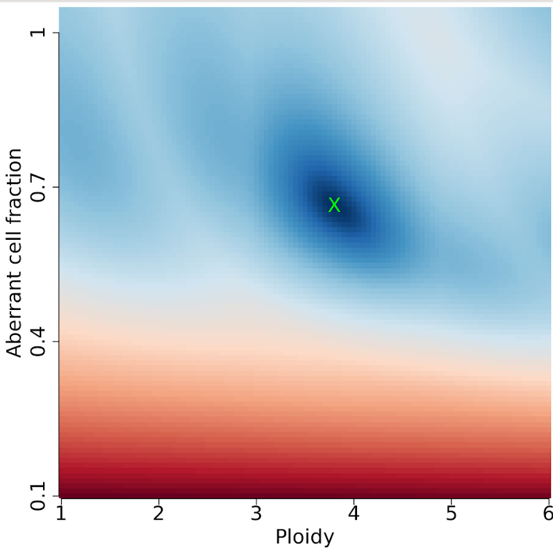
19-4 Sunrise plot (NSLC-AKVX-TTP1-A-1-1-D-A81L-36.sunrise.png)

Sunrise plot offers the possible solutions in the expected combination of tumor purity/ploidy. Generally, the upper section of the sunrise plot is predominantly blue with a sloped delineation at the red/blue border. The blue indicates a good solution; red indicates a bad solution.

Our result is slightly unusual because it is a clean result with one observed combination of purity/ploidy.

19-5 Ploidy & Purity (NSLC-AKVX-TTP1-A-1-1-D-A81L-36.samplestatistics.txt)

vim /data/$USER/practical_session_7/ASCAT_NGS/Expect_result_ASCAT_NGS/NSLC-AKVX-TTP1-A-1-1-D-A81L-36.samplestatistics.txt

NormalContamination 0.194866005269865
Ploidy 4.0700637770928
rho 0.67
psi 3.8
goodnessOfFit 98.6380966709408
GenderChr Y
GenderChrFound N

• Ploidy: Tumor ploidy (average copy number state across the genome)
• rho: Tumor purity (Aberrant cell fraction)
• psi: Internal ASCAT ploidy parameter
• goodnessOfFit: Confidence metric

Comparing ASCAT and FACETS results

SCNA Profiles Plot from FACETS algorithms (Black: Total SCNAs; Red: Minor SCNAs)

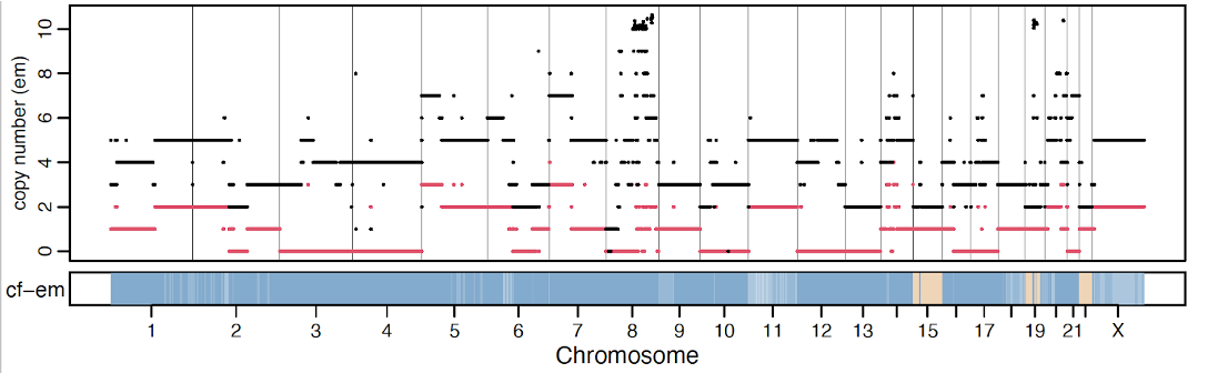
SCNA Profiles Plot from ASCAT algorithms (Red: Major SCNAs; Green: Minor SCNAs)

Purity and Ploidy

Purity/ploidy from FACETS:

sample  purity  ploidy
Test    0.640416509675053       4.02317905682627

Purity/ploidy from ASCAT algorithms:

Ploidy 4.0700637770928
rho 0.67

We can see results from the two algorithms are very consistent. There can be high power for different algorithms to accurately detect SCNAs in the current sample.

Apply GISTIC2 for identification of statistically significant frequent copy number alteration

Somatic copy number alterations are distributed across the whole genome, however only a few ‘driver’ alterations can promote cancer development. How to distinguish those driver SCNAs from random passenger SCNAs is a critical question.

GISTIC is a well known tool for Genomic Identification of Significant Targets in Cancer. The method identifies recurrent focal events which are more likely to be drivers of tumorigenesis based on their frequency. Through GISTIC analysis we can get a list of significant SCNA regions. According to the latest statistics from Google scholar, this tool has been cited by ~2500 times, since its first publication in 2011.

20. Go back from the current working directory to practical_session_7, where $USER is the current user’s username.

cd /data/$USER/practical_session_7/

21. Create a dir “GISTIC” for running this tool

mkdir GISTIC
cd GISTIC

22. Copy the file Session_7_3_GISTIC_sbatch.sh to the current working directory.

cp /data/classes/DCEG_Somatic_Workshop/Practical_session_7/Gistic/Session_7_3_GISTIC_sbatch.sh .

23. Submit the file Session_7_3_GISTIC_sbatch.sh to a workload manager (e.g., SLURM) using the sbatch command.

sbatch --cpus-per-task=2 --mem=20g --time=7:27:27 Session_7_3_GISTIC_sbatch.sh

You can always check the status of the jobs by typing:

squeue -u $USER

sjobs

24. Have a closer look at our sbatch script:

vim /data/classes/DCEG_Somatic_Workshop/Practical_session_7/Gistic/Session_7_3_GISTIC_sbatch.sh

#!/bin/bash
#SBATCH -o sbatch_output.txt
#SBATCH -e sbatch_error.txt

module load gistic


basedir=`pwd`/output
mkdir $basedir
InputDir=/data/classes/DCEG_Somatic_Workshop/Practical_session_7/Gistic/Input_Data
segfile=$InputDir/sherlock_gistic_input.txt
markersfile=$InputDir/hg19_markers.txt
refgenefile=$InputDir/hg19.mat


gistic2 \
 -b $basedir \
 -seg $segfile \
 -mk $markersfile \
 -refgene $refgenefile \
 -genegistic 1 \
 -smallmem 1 \
 -broad 1 \
 -brlen 0.5 \
 -conf 0.90 \
 -armpeel 1 \
 -savegene 1 \
 -gcm extreme

# sbatch --cpus-per-task=2 --mem=20g --time=3:27:27 Session_7_3_GISTIC_sbatch.sh

• Line 1 is the header of this script, to tell biowulf it is generated in the bash program.
• Line 2 and Line 3 is used to produce log file to summarise output and error
• Line 5 is used to load gistic as well as the required running environment
• Line 8 to Line 13 is used to define the absolute path of input & output, and required reference files.
• Line 16 to Line 28 is used to run gistic program for identification of significant SCNA regions.

Input

Segmentation File (-seg)

The segmentation file contains the segmented data for all the samples identified by different SCNA callers, with six column separated by “tab”

Example of Segmentation File:

NSLC-0001-T01	1	776546	31247028	16000	1.64508
NSLC-0001-T01	1	31247089	60488008	12760	1.5162
NSLC-0001-T01	1	60489461	145095590	30127	1.10095
NSLC-0001-T01	1	145095756	249214082	54411	1.54324
NSLC-0001-T01	2	23368	55711409	32535	1.40855

1. Sample: sample name
2. Chromosome: chromosome number
3. Start Position: segment start position, in bases
4. End Position: segment end position, in bases
5. Num Markers: number of markers in segment
6. Seg.CN: log2()-1 of copy number

Markers File (-mk)

The markers file identifies the marker positions used in the original dataset from array or capture experiments for segmentation. Before GISTIC Version 2.0.23, the markers file is a required item. Now, it has been updated to an optional input. If excluded, markers are generated as uniformly as possible using the maxspace input parameter.

Example of markers File:

SNP_1_762601	1	762601
SNP_1_762843	1	762843
SNP_1_762947	1	762947
SNP_1_763091	1	763091
SNP_1_764191	1	764191

The markers file is a three column, tab-delimited file. The column headers are:

1. Marker Name
2. Chromosome
3. Marker Position (in bases)

Reference Genome File (-refgene) REQUIRED

The reference genome file contains information about the location of genes and cytobands of the genome. Reference genome files are created in mat format and are not viewable with a text editor. The GISTIC has provided several pre-built reference genomes: hg16.mat, hg17.mat, hg18.mat, hg19.mat and hg38.mat.

Output Files

25. To explore the expected results while the job is running, copy the result files from the expected result folders in your biowulf directory:

cp -r /data/classes/DCEG_Somatic_Workshop/Practical_session_7/Expect_result/Expect_result_GISTIC .

Explore GISTIC output

25-1 All Lesions File (all_lesions.conf_90.txt, where 90 is the confidence level)

The all lesions file summarises the results from the GISTIC run. It contains data about the significant regions of amplification and deletion as well as which samples are amplified or deleted in each of these regions.

vim /data/$USER/practical_session_7/GISTIC/Expect_result_GISTIC/all_lesions.conf_90.txt

Example Output File:

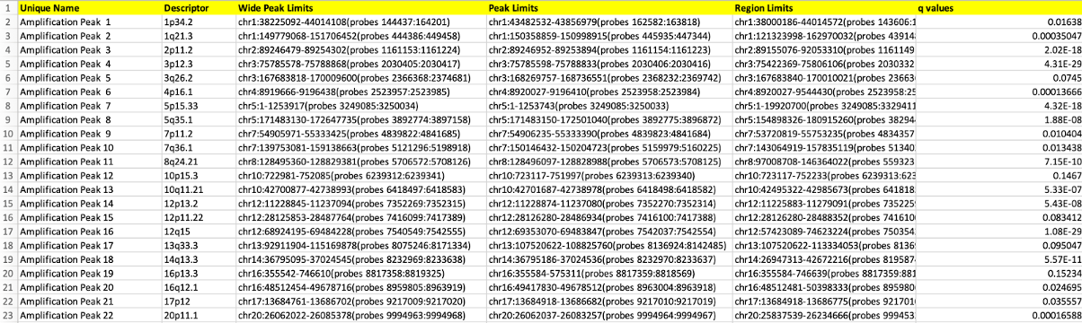
Columns 1-8 present the data about the significant regions as follows:

1. Unique Name: A name assigned to identify the region
2. Descriptor: The genomic location of that region.
3. Wide Peak Limits: The boundaries of all genomic coordinates and marker indices.
4. Peak Limits: The boundaries of the region of maximal amplification or deletion.
5. Region Limits: The boundaries of the entire significant region of amplification or deletion.
6. q-values: The q-value of the peak region.
7. Residual q-values: The q-value of the peak region after removing (“peeling off”) amplifications or deletions that overlap other, more significant peak regions in the same chromosome.
8. Broad or Focal: Identifies whether the region reaches significance due primarily to broad events (called “broad”), focal events (called “focal”), or independently significant broad and focal events (called “both”).

25-2. Amplification Genes File (amp_genes.conf_90.txt, where 90 is the confidence level)

vim /data/$USER/practical_session_7/GISTIC/Expect_result_GISTIC/amp_genes.conf_90.txt

The amp genes file contains columns for each amplification peak identified in the GISTIC analysis.

Example File:

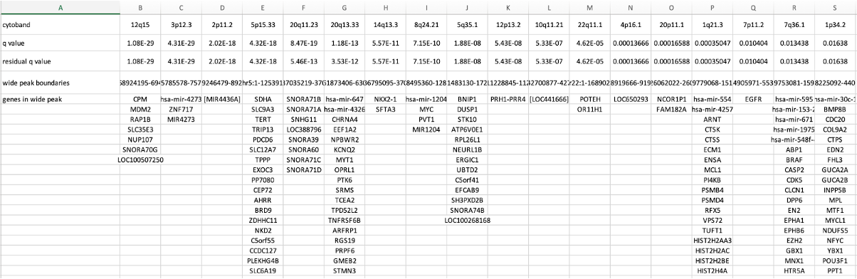
The top rows are:

1. cytoband
2. q-value
3. residual q-value
4. wide peak boundaries
5. Genes located at each significantly SCNA regions

25-3. Deletion Genes File (del_genes.conf_90.txt, where 90 is the confidence level)**

vim /data/$USER/practical_session_7/GISTIC/Expect_result_GISTIC/del_genes.conf_90.txt

The del genes file contains columns for each deletion peak identified in the GISTIC analysis. The file format for del genes file is identical to the format for amp genes file.

Example File:

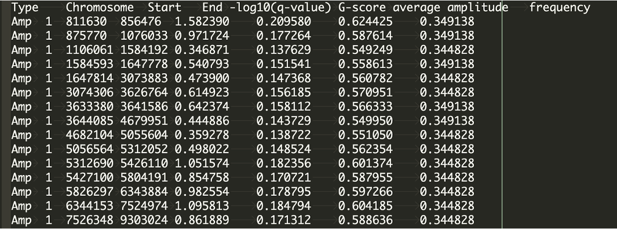
25-4. Gistic Scores File (scores.gistic)

The scores file presents the q-values [presented as -log10(q)], G-scores, average amplitudes among aberrant samples, and frequency of all segmentations across the genome for both amplifications and deletions.

vim /data/$USER/practical_session_7/GISTIC/Expect_result_GISTIC/scores.gistic

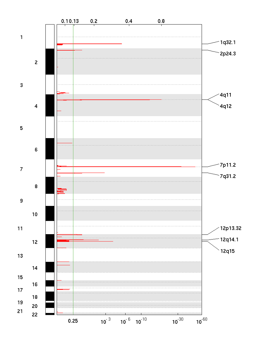
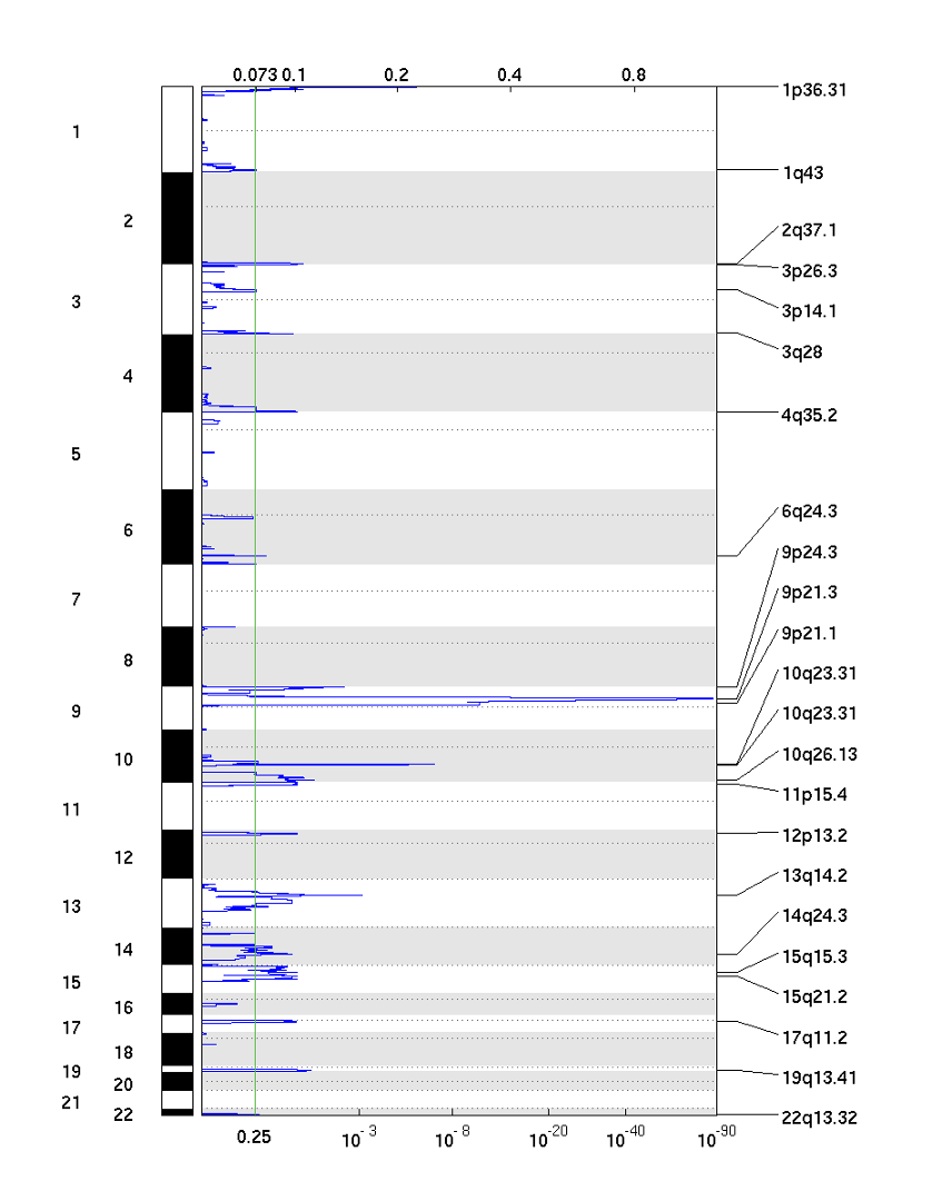
25-5. GISTIC plot with Amplification Score (amp_qplot.pdf)

The amplification pdf is a plot of the G-scores (top) and q-values (bottom) with respect to amplifications for all markers over the entire region analysed.

25-6. GISTIC plot with deletion Score (del_qplot.pdf)

The deletion pdf is a plot of the G-scores (top) and q-values (bottom) with respect to deletions for all markers over the entire region analyzed.

​​This is a general description to run the GISTIC algorithm. To learn more detailed information and some advanced usage, you can check the official document with the following link: (https://broadinstitute.github.io/gistic2/)

Identification of somatic copy number alteration signatures

Introduction to the 21 breast cancers project

The dataset for today’s practical session is the whole genome sequencing data from the “Life History of 21 Breast Cancers” study, led by Dr. Nik-Zainal and colleagues at the Wellcome Trust Sanger Institute. This is a significant study in the field of cancer genomics, in which the researchers applied whole genome sequencing technology to 21 breast cancers with an average sequencing depth of 30-40X and analyzed somatic mutations and signatures to understand the life histories of these cancers. For today’s session, we will be using the cleaned mutation calling data from this study.

Bioinformatics tools

• SigProfilerMatrixGenerator: creates mutational matrices for somatic mutations. This classifies large-scale alterations such as SCNAs and SVs as well as single base substitutions (SBSs), double base substitutions (DBSs), and insertions/deletions (IDs) according to a predefined schema. In the output matrix, rows are features and columns are samples. This matrix is amenable to decomposition techniques such as NMF. We will use a 48 channel classification scheme developed by Steele and (https://www.nature.com/articles/s41586-022-04738-6) and implemented by Khandekar et. al. (https://www.biorxiv.org/content/10.1101/2023.02.03.527015v1).
• SigProfilerExtractor: Performs extraction of mutational signatures from somatic mutational matrix created by SigProfilerMatrixGenerator. This can be followed by decomposition analysis based on a set of reference signatures available in COSMIC. The main outputs are the signatures matrix (shows a signatures preference for specific features) and activities matrix (which contains the activities of each signature in each sample ).
• SigProfilerPlotting: Visualize various types of mutational patterns and mutational signatures in cancer genomes. This tool will be used to visualize all the mutational matrices generated by the SigProfilerMatrixGenerator as well as mutational signatures from the output of SigProfilerExtractor.

Generate SCNA matrix and identify SCNA Signatures

Make sure that your interactive session is ready

26. Create a folder for analysis/results and copy the relevant scripts we will use to your folder

cd /data/$USER/
mkdir SCNA_Signatures
cd SCNA_Signatures

cp /data/classes/DCEG_Somatic_Workshop/Practical_session_7/SCNA_Signatures/session_7_sbatch_4_extract_SCNA_Sigantures.sh /data/$USER/SCNA_Signatures

cp /data/classes/DCEG_Somatic_Workshop/Practical_session_7/SCNA_Signatures/extract_signatures.py .

27. Install SigProfiler suite of tools for mutational signature analysis:

module load python/3.9
pip install SigProfilerMatrixGenerator #matrix generation
pip install SigProfilerPlotting #visualization
git clone https://github.com/AlexandrovLab/SigProfilerExtractor.git
cd SigProfilerExtractor/
pip install .
cd /data/$USER/SCNA_Signatures

28. Clone SigProfilerMatrixGenerator repo to generate SCNA matrices:

git clone https://github.com/AlexandrovLab/SigProfilerMatrixGenerator.git

29. Let’s take a closer look at our input file, which is located at:

less /data/classes/DCEG_Somatic_Workshop/Practical_session_7/SCNA_Signatures/Input_Data/all.breast.ascat.summary.sample.tsv

This is a segmentation file generated by the SCNA caller ASCAT-NGS.

It has eight columns and represents allele-specific SCNA’s:

1. Sample ID
2. Chromosome
3. Start Position
4. End position,
5. Normal TCN,
6. Normal BCN,
7. Tumor TCN
8. Tumor BCN

SigProfilerMatrixGenerator provides support for various SCNA callers (ASCAT, ABSOLUTE Sequenza, FACETS, Battenberg, and PURPLE.).

30. Next, generate the CNV matrix with sample ASCAT data using a simple one-liner:

python ./SigProfilerMatrixGenerator/SigProfilerMatrixGenerator/scripts/CNVMatrixGenerator.py ASCAT_NGS /data/classes/DCEG_Somatic_Workshop/Practical_session_7/SCNA_Signatures/Input_Data/all.breast.ascat.summary.sample.tsv 560-Breast /data/$USER/SCNA_Signatures

The output from SigProfilerMatrixGenerator should look like this:

31. Next, we will extract signatures using SigProfilerExtractor. In order to do this, Submit the script session_7_sbatch_4_SCNA_Sig.sh to a workload manager (e.g., SLURM) using the sbatch command.

sbatch --cpus-per-task=8 --mem=8g --time=3:00:00 session_7_sbatch_4_SCNA_Sig.sh

Note: the –cpus-per-task, –mem, and –time flags are options that specify the number of CPU cores, amount of memory, and maximum runtime for the job, respectively.

You can check the job running status using sjobs **or **squeue -u $USER.

The script will run for about 20 minutes.

32. To save time, let’s explore the expected results while the job is running. Copy the result files from the expected result folders in your biowulf directory:

cp -r /data/classes/DCEG_Somatic_Workshop/Practical_session_7/SCNA_Signatures/SCNA_Signatures_Expected_Result .

33. After mounting the HPC drive, users can check the expected result folder in their local system.

Let’s take a closer look at our working script extract_signatures.py:

less /data/classes/DCEG_Somatic_Workshop/Practical_session_7/SCNA_Signatures/extract_signatures.py

from SigProfilerExtractor import sigpro as sig

# encoding=utf8
import argparse
import os
import re


# NMF RUNS:-

# **minimum_signatures**: A positive integer, optional. The minimum number of signatures to be extracted. The default value is 1

# **maximum_signatures**: A positive integer, optional. The maximum number of signatures to be extracted. The default value is 10

# **nmf_replicates**: A positive integer, optional. The number of iteration to be performed to extract each number signature. The default value is 100

# **resample**: Boolean, optional. Default is True. If True, add poisson noise to samples by resampling.

# **random_seeds**: Boolean. Default is True. If True, then the seeds for resampling will be random for different analysis.
#               If False, then resampling will be identical for repeated analysis.

# NMF RUNS:-

# **matrix_normalization**: A string. Method of normalizing the genome matrix before it is analyzed by NMF. Default is "log2". Other options are "gmm", "100X" or "no_normalization".

# **nmf_init**: A String. The initialization algorithm for W and H matrix of NMF. Options are 'random', 'nndsvd', 'nndsvda', 'nndsvdar' and 'alexandrov-lab-custom'
#           Default is 'alexandrov-lab-custom'

# **precision**: A string. Values should be single or double. Default is single.

# **min_nmf_iterations**: An integer. Value defines the minimum number of iterations to be completed before NMF converges. Default is 2000.

# **max_nmf_iterations**: An integer. Value defines the maximum number of iterations to be completed before NMF converges. Default is 200000.

# **nmf_test_conv**: An integer. Value definer the number number of iterations to done between checking next convergence. Default is 1000.

# **nmf_tolerance**: A float. Value defines the tolerance to achieve to converge. Default is 1e-8.

minimum_signatures=1
maximum_signatures=3
matrix_normalization="gmm"
nmf_init="random"
reference_genome="GRCh38"
opportunity_genome = "GRCh38"
context_type = "default"
exome = False
nmf_replicates=5
resample = True
batch_size=1
cpu=-1
gpu=False
precision= "single"
seeds= "random"
min_nmf_iterations= 10000
max_nmf_iterations=1000000
nmf_test_conv= 10000
nmf_tolerance= 1e-15
nnls_add_penalty=0.05
nnls_remove_penalty=0.01
de_novo_fit_penalty=0.02
initial_remove_penalty=0.05
refit_denovo_signatures=False
clustering_distance="cosine"
export_probabilities=True
make_decomposition_plots=True
stability=0.9
min_stability=0.2
combined_stability=1.0
get_all_signature_matrices=True
input_type = "matrix"


if __name__ == "__main__":
        project = "560-breast-ASCAT"
        data = "/data/classes/DCEG_Somatic_Workshop/Practical_session_7/SCNA_Signatures/560-Breast.CNV48.matrix.tsv"
        sig.sigProfilerExtractor(input_type,
                         project,
                         data, reference_genome=reference_genome,
                         opportunity_genome=opportunity_genome,
                         context_type=context_type,
                         exome=exome,
                         minimum_signatures=minimum_signatures,
                         maximum_signatures=maximum_signatures,
                         nmf_replicates=nmf_replicates,
                         resample=resample,
                         batch_size=batch_size,
                         cpu=cpu,
                         gpu=gpu,
                         nmf_init=nmf_init,
                         precision=precision,
                         matrix_normalization=matrix_normalization,
                         seeds=seeds,
                         min_nmf_iterations=min_nmf_iterations,
                         max_nmf_iterations=max_nmf_iterations,
                         nmf_test_conv=nmf_test_conv,
                         nmf_tolerance=nmf_tolerance,
                         nnls_add_penalty=nnls_add_penalty,
                         nnls_remove_penalty=nnls_remove_penalty,
                         de_novo_fit_penalty=de_novo_fit_penalty,
                         initial_remove_penalty=initial_remove_penalty,
                         refit_denovo_signatures=refit_denovo_signatures,
                         clustering_distance=clustering_distance,
                         export_probabilities=export_probabilities,
                         make_decomposition_plots=make_decomposition_plots,
                         stability=stability,
                         min_stability=min_stability,
                         combined_stability=combined_stability,
                         get_all_signature_matrices=get_all_signature_matrices)

Key arguments to SigProfilerExtractor:

minimum_signatures=1
maximum_signatures=3
matrix_normalization="gmm"
nmf_init="random"
reference_genome="GRCh38"
opportunity_genome = "GRCh38"
context_type = "default"
exome = False
nmf_replicates=5

...

if __name__ == "__main__":
        project = "560-breast-ASCAT"
        data = "/data/classes/DCEG_Somatic_Workshop/Practical_session_7/SCNA_Signatures/560-Breast.CNV48.matrix.tsv"
        sig.sigProfilerExtractor(input_type,
                         project,
                         data, reference_genome=reference_genome,
                         opportunity_genome=opportunity_genome,
                         context_type=context_type,
                         exome=exome,
                         minimum_signatures=minimum_signatures,
                         maximum_signatures=maximum_signatures,
                         nmf_replicates=nmf_replicates,
                         resample=resample,
                         batch_size=batch_size,
                         cpu=cpu,
                         gpu=gpu,
                         nmf_init=nmf_init,
                         precision=precision,
                         matrix_normalization=matrix_normalization,
                         seeds=seeds,
                         min_nmf_iterations=min_nmf_iterations,
                         max_nmf_iterations=max_nmf_iterations,
                         nmf_test_conv=nmf_test_conv,

Explore the output from SigProfilerExtractor

Due to the limited time, here we have only provided a brief overview of the main directories. For a complete description of all output, please refer to the official documentation.

cd /data/classes/DCEG_Somatic_Workshop/Practical_session_7/SCNA_Signatures/SCNA_Signatures_Expected_Result/SigProfilerExtractor/

SigProfilerExtractor
├── CNV48
├── JOB_METADATA.txt
└── Seeds.txt

• JOB_METADATA.txt contains metadata about this job, including: operating system, Python and Package Versions, Analysis Progress and Job Status.
• Seeds.txt contains an ID which is used to initialize a random number generator for iterating simulation.
• subdirectory CNV48 is the major output of specific mutational context extracted by SigProfilerExtractor, including:
  • All_Solutions subdirectory
  • Suggested_Solution subdirectory
  • All_solutions_stat.csv
  • SBS96_selection_plot.pdf
  • Samples.txt

Subdirectory CNV48/All_Solutions contains the results from running de novo extractions at each rank within the range of the input maximum signature numbers. As our maximum_signatures is 3, there are three subdirectories, beginning with CNV48_1_Signatures to CNV48_3_Signatures.

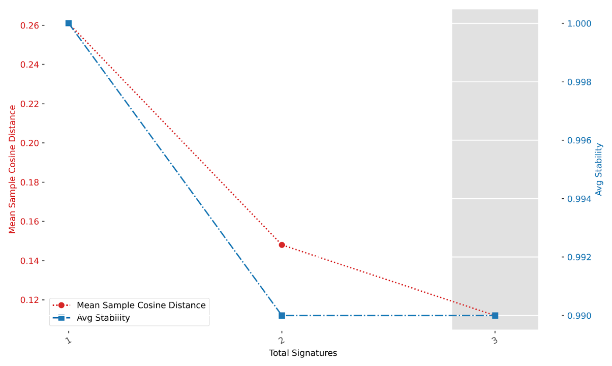
CNV48_selection_plot.pdf contains a plot between the mean sample cosine distance and the average stability. The gray bar indicates the optimal number of signatures selected by SigProfilerExtractor.

CNV48/Samples.txt contains the initial input matrix you provided for signature extraction.

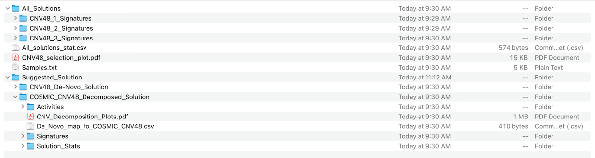
Subdirectory CNV48/Suggested_Solution subdirectory contains the optimal solution, also the result we need. Let’s go to the subdirectory CNV48_De-Novo_Solution and view it:

cd /data/classes/DCEG_Somatic_Workshop/Practical_session_7/SCNA_Signatures/SCNA_Signatures_Expected_Result/SigProfilerExtractor/CNV48/Suggested_Solution/CNV48_De-Novo_Solution

less ./Signatures/CNV48_De-Novo_Signatures.txt

We can see that two de novo signatures (CNV48A, CNV48B) were extracted from the input mutational matrix. This matrix represents a probability distribution that characterizes each signature.

Open CNV48_De-Novo_CNV48_signatures.pdf, in which you can find the visualization of these signatures.

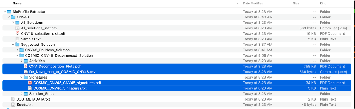
Let’s view the file COSMIC_CNV48_Activities.txt. This matrix contains the activity of each signature in each sample (i.e the # of mutations attributed to each signature in each sample).***

cd /data/classes/DCEG_Somatic_Workshop/Practical_session_7/SCNA_Signatures/SCNA_Signatures_Expected_Result/SigProfilerExtractor/CNV48/Suggested_Solution/CNV48_De-Novo_Solution

less ./Activities/CNV48_De-Novo_Activities_refit.txt

Check the results of the mutational signature decomposition as highlighted in blue in the following screenshot.

De_Novo_map_to_COSMIC_CNV48.csv contains data on how the de novo extracted signatures are decomposed using the COSMIC reference signatures. Additionally, it also contains information on the L1 error %, L2 error %, KL divergence, cosine similarity, and correlation of this decomposition.

CNV_Decomposition_Plots.pdf There are two plots to the left of the curly brace. One is the original de novo signature plot and the other is the reconstruction of the de novo signature. On the right side of the curly brace are the COSMIC signatures that the de novo signature is decomposed to.

COSMIC_CNV48_CNV48_signatures.pdf, in which you can find the visualizations of these COSMIC reference signatures.

Detailed instructions on using SigProfiler tools can be found here:

• SigProfilerMatrixGenerator
• SigProfilerExtractor
• SigProfilerPlotting