TPM normalization
This section includes the method for TPM normalization. This normalization provides counts per length of transcript (kilobases) per million reads mapped. This method accounts for sequencing depth and gene length.
This normalization will be carried out in R. Make sure you have installed and loaded all of the necessary packages (see Preparation under Practical tab).
Also make sure that you have downloaded the zip file (in the Practical tab) that contains all of the necessary files for this process. Unzip this file and select the Practical_session_11_normalization_DE.R file from the scripts folder. This will open a window in RStudio.
Make sure you are in the correct directory by using the getwd() command. The directory should be:
Mac
/Users/[username]/Downloads/Practical_session_11/
Windows
"C:/Users/[username]/Downloads/Practical_session_11/
If you are not, use the setwd() command:
setwd("/Users/kleinam/Documents/epi_studies_course/Practical_session_11/")
First, we will read in the necessary files to run the TPM normalization. These include a sample annotation file (Practical_11_samples_clinical.txt), the htseq raw count data (Practical_11_candidate_TP53_cnt_GeneName_N20_recode.txt) and gene length data (gencode.v35.annotation.length.featureCounts.ByGeneName.txt).
This is covered in lines 37-45 in our code:
# read in sample annotations
metadata <- read_delim('Practical_11_samples_clinical.txt')
# read in raw counts output from htseq
htseq_output <- read_delim('Practical_11_htseq_counts.txt') %>% data.frame()
# rename UID to gene_name (to be used later)
htseq_output <- dplyr::rename(htseq_output, gene_name = UID)
# set row names to gene names and remove the gene_name column (the first column in the dataframe)
rownames(htseq_output) <- htseq_output$gene_name
htseq_output <- htseq_output %>% select(-1)
gene_lengths <- read_delim('gencode.v35.annotation.length.featureCounts.ByGeneName.txt')
We can look at the first few lines of each of these files to get an idea of the format of each:
head(metadata) %>% View()

head(htseq_output) %>% View()
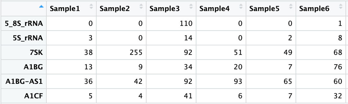
head(gene_lengths) %>% View()

Next, we filter out any genes with extremely low counts (<10) using the rowSums() command.
# filter out any genes where the read counts across samples are not greater than or equal to 10
htseq_output <- htseq_output %>%
  dplyr::filter(rowSums(.) >= 10)
# add gene_name column back in and reset rownames to NULL (all columns to calculate rowSums needed to be numeric- gene_name was not numeric)
htseq_output <- htseq_output %>% mutate(gene_name = rownames(htseq_output) ,.before = 1)
rownames(htseq_output) <- NULL
Now, we will join the htseq raw count data with the gene length data so that we can divide our raw counts by the corresponding gene length.
# filter out any genes where the read counts across samples are not greater than or equal to 10
htseq_output <- htseq_output %>%
  dplyr::filter(rowSums(.) >= 10)
# add gene_name column back in and reset rownames to NULL (all columns to calculate rowSums needed to be numeric- gene_name was not numeric)
htseq_output <- htseq_output %>% mutate(gene_name = rownames(htseq_output) ,.before = 1)
rownames(htseq_output) <- NULL
# join htseq data with gene length data so we can account for gene length in normalization
htseq_output <- htseq_output %>% left_join(gene_lengths)
# make the data frame of wider format to divide each count by the corresponding gene length
htseq_output <- htseq_output %>% pivot_longer(cols = starts_with('Sample'))
# divide each count by corresponding gene length
htseq_output <- htseq_output %>% mutate(gene_length_norm = value/length)
# values that have now been divided by gene length; put back into dataframe where each sample is a column - Sample RPKs
htseq_tmp <- htseq_output %>% pivot_wider(names_from = name, values_from = gene_length_norm) %>% group_by(gene_name) %>% summarise(across(starts_with("Sample"), ~sum(., na.rm = TRUE)))
Now our counts are in Reads Per Kilobase (RPK). We next find the total RPK for each sample by adding up all of the RPKs per sample.
# total RPKs per each sample
htseq_tmp2 <- htseq_output %>% group_by(name) %>% summarise(sum(gene_length_norm)) %>% mutate(total = `sum(gene_length_norm)`) %>% select(-2)
Then we find the scaling factor to be used for each sample by taking the total RPK per sample and dividing it by 1,000,000.
# calculate scaling factor by taking total RPK for a sample and dividing it by 1000000 (i.e. transcripts per MILLION)
htseq_tmp2 <- htseq_tmp2 %>% mutate(scaling_factor = total/1000000)
Finally, we take the scaling factor calculated for each sample and divide the RPKs (i.e. reads that have been normalized for gene length) from step xx to calculate the normalized counts.
# divide each sample by the appropriate scaling factor determined in the previous line of code
# R loop to divide each column by the correct value
sample_names <- paste0('Sample',rep(1:20))
i <- 1
for(each in sample_names){
sample_name <- paste0('Sample',i)
print(sample_name)
#scaling_factor <- htseq_tmp2$scaling_factor[which(htseq_tmp2$name == 'Sample1')]
scaling_factor <- htseq_tmp2$scaling_factor[which(htseq_tmp2$name == sample_name)]
htseq_tmp[,sample_name] <- htseq_tmp[,sample_name]/scaling_factor
i <- i + 1

}
Then, we save the normalized counts to a file.
# save the normalized counts to a file
htseq_normalized_tpm <- htseq_tmp
write_delim(htseq_normalized_tpm, file= 'htseq_normalized_tpm.csv',delim = ',')