Presenters: Wei Zhao, Alyssa Klein
In today’s practical session, we will be focusing on the first step of the RNA-Seq data analysis workflow, raw gene expression quantification. The steps we will be covering today include sequence alignment, post-alignment quality assessment, visualization of the alignment, and transcript quantification.
Overview of Data
Today’s session will focus on two RNA-Seq tumor samples. Both samples are from the Environment And Genetics in Lung cancer Etiology (EAGLE) study, which includes smokers with lung cancer. While we will mainly be working with the good quality sample- CSP97520- in our workflow today, we will be comparing it to the bad quality sample-CSP107316- as a reference.
Sequencing Data Quality Check
Before running the STAR aligner, it is important that we check the overall quality of our two samples. In session three, you will recall that we ran FastQC and MultiQC to look at the quality of the whole-genome sequencing (WGS) data. Today, we have already run FastQC to save time, and so we are going to quickly generate the MultiQC report and highlight what are considered the 5 main FastQC measures:
- Per base sequence quality
- Per sequence quality scores
- Per sequence GC content
- Per base N content
- Overrepresented sequences
It is a good benchmark that samples pass at least 3 of these 5 measures, as discussed here in a paper by the PCAWG Consortium: https://www.nature.com/articles/s41586-020-1970-0.
Before doing anything else, mount to your data directory as we have several times throughout the course. We will need to look at output files on your local machine. If you need a refresher, use the following link: https://hpc.nih.gov/docs/helixdrive.html.
Run MultiQC
First, let’s copy the FastQC output to your data directory.
1. Log onto Biowulf using the following command, substituting your username where it says [username].
ssh [username]@biowulf.nih.gov
2. Set up an interactive session using the following command:
sinteractive --mem=4g --cpus-per-task=2 --time=4:00:00
This sets up the default interactive node with 2 CPUs and 4 GB memory, for 4 hours.
3. Change the directory to the data directory:
cd /data/$USER
4. Create a directory for this practical session using the following command:
mkdir practical_session_10
5. Move to that directory so that it becomes your working directory and check that you are now in this directory:
cd practical_session_10
pwd
6. Copy the FastQC output for both samples to practical_session_10:
cp -R /data/classes/DCEG_Somatic_Workshop/Practical_session_10/quality_checks .
7. After copying this quality_checks folder, move into this directory and use the tree command:
cd quality_checks
tree
.
├── CSP107316_1_fastqc.html
├── CSP107316_1_fastqc.zip
├── CSP107316_2_fastqc.html
├── CSP107316_2_fastqc.zip
├── CSP97520_1_fastqc.html
├── CSP97520_1_fastqc.zip
├── CSP97520_2_fastqc.html
├── CSP97520_2_fastqc.zip
├── insert_size_histogram.pdf
├── insert_size_metrics.txt
└── Picard_RNA_Metrics.txt
You will see several FastQC output files. There is a zip file and a html file per R1 and R2 for each sample. This is due to this sequencing data being paired-end sequencing, where there is a Read1 (R1) and a Read2 (R2), or mates, for each sample. R1 is referred to as the first mate, and R2 is referred to as the second mate.
FastQC runs each of the mate files separately, leading to each sample to have two FastQC output files.
8. In order to run MultiQC, we first load the module using the following command:
module load multiqc
You will see the following appear to show that the module had been loaded:
[+] Loading singularity  3.10.5  on cn4329
[+] Loading multiqc  1.14
9. Use the following command to run MultiQC using the FastQC output for both samples:
multiqc --title "S10_RNA_quality" . --ignore Picard_RNA_Metrics.txt --ignore insert_size_histogram.pdf --ignore insert_size_metrics.txt
The parameters used to run MultiQC are explained below:
- title- the name of the report that will be generated
- . - sets the analysis directory to the current directory (quality checks)
- ignore- ignores specific files that we do not wish to include in the report
This should take less than 10 seconds to run. When it is finished, you will see a folder and a file have been generated:
- S10_RNA_quality_multiqc_report_data
- S10_RNA_quality_multiqc_report.html
We will focus on S10_RNA_quality_multiqc_report.html.
10. Access the report (S10_RNA_quality_multiqc_report.html) from the data directory that you mounted to at the beginning of the session, or you can click here to access the report.
Copy all files needed for practical session
Before we move on to explore the MultiQC output, we are going to set up all of the files needed for this session to be copied over to the practical_session_10 folder you have created:
cd ..
cp -R /data/classes/DCEG_Somatic_Workshop/Practical_session_10/scripts .
cp -R /data/classes/DCEG_Somatic_Workshop/Practical_session_10/quantification .
cp -R /data/classes/DCEG_Somatic_Workshop/Practical_session_10/STAR_output .
Explore MultiQC Output
We can start by looking at the sample summary at the top of the report. You will notice that I have color-coded the samples to make them easier to distinguish throughout the report. You may do this as well using the toolbox option on the right of the report, but it is not necessary.
At a glance, here we see a higher percentage of duplicates and a higher number of sequencing reads in sample CSP97520.
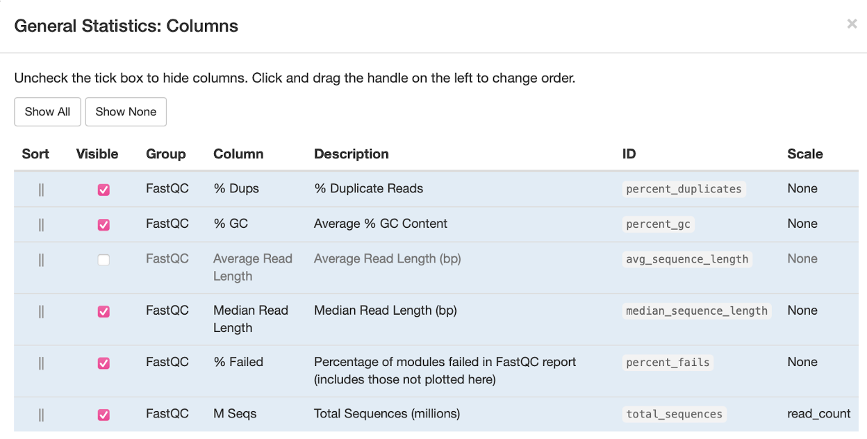
For reference, you can click on Configure Columns to see what each column means. You will see something that looks like this:
11. As previously mentioned, we are going to quickly highlight what are considered the 5 most important FastQC measures:
- Per base sequence quality
- Per sequence quality scores
- Per sequence GC content
- Per base N content
- Overrepresented sequences
We will review the plots and their meaning below.
Per base sequence quality
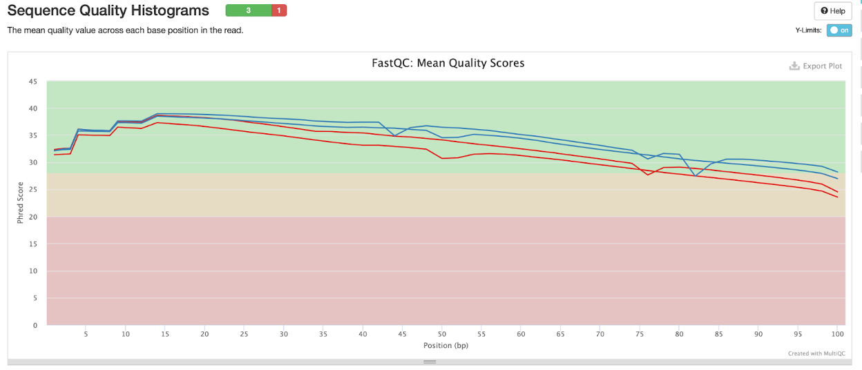
Here we can see that the sample CSP97520 has a much more consistent and high sequence quality at base position in the read compared to the CSP107316 sample.
Per sequence quality scores
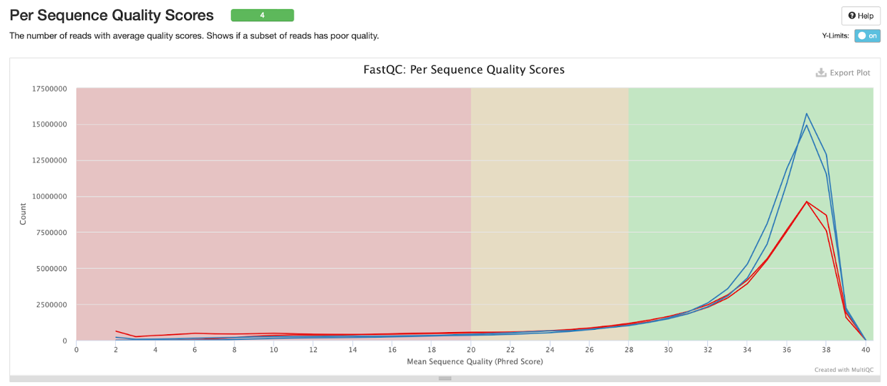
In the plot below we see that the per sequence quality scores are similar for both samples, at about 36 for both R1 and R2 of both samples.
Per sequence GC content
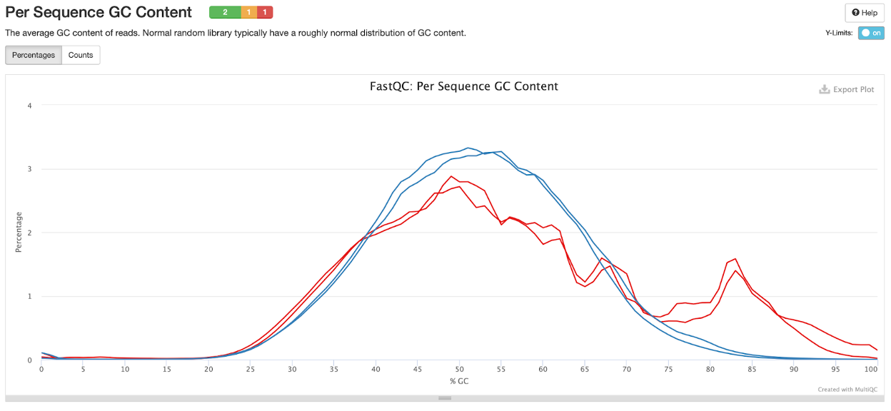
The plot below illustrates the GC content in R1 and R2 for both samples. We see that the GC content in the CSP97520 sample is right around 50% in about 3% of the reads, whereas we see two peaks for GC content in the CSP107316 sample, with about 1.5% of reads with much higher GC content (~80-85%). It is important to pay attention to GC content because it can lead to gene quantification bias in downstream analysis (i.e. differential expression analysis).
Per base N content
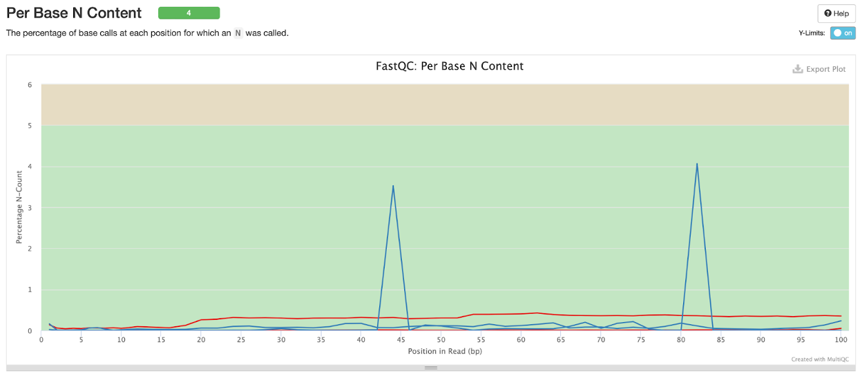
‘N’ is when the base at a given position was not identified as any of the four (A, T, C, or G). Here we see a slightly higher percentage N-count in the CSP97520 sample between base position 40-45 and 80-85, but both mates for both samples passed this feature.
Overrepresented sequences
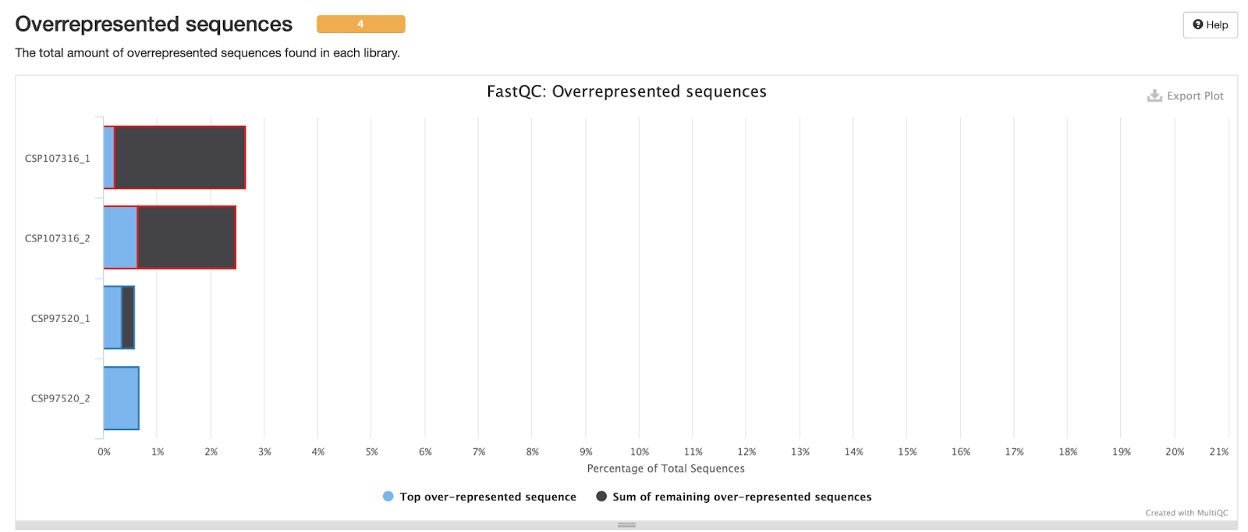
Lastly, we check the overrepresented sequences in both R1 and R2 of our samples. We see that there is a greater percentage of these sequences in the CSP107316 sample. As mentioned in the lecture, most RNA-seq pipelines do not include computational deduplication. This is typically carried out by sequence of comparison or aligned coordinates. Short transcripts and very highly expressed transcripts (common in some species) will contribute the majority of biological ‘duplicates’.
Based on this report, both samples are passed to run through alignment due to their passing (warnings included) at least 3 of the 5 measures discussed above.
Trimming or No Trimming?
When talking about RNA-Seq data and its subsequent analysis, you will often find that the workflows include trimming before alignment. Trimming is when the reads are ‘cleaned’ by removing adapter sequences (and oftentimes low quality bases).
However, most of the popular aligners no longer require adapter trimming for mRNA-seq. However, it depends on the RNA type, as well as the purpose of your study. With regard to RNA type, trimming should still be done for shorter reads experiments, such as miRNA-seq. With regard to study purpose, if doing sequencing for counting applications (such as differential gene expression (DGE) RNA-seq analysis), read trimming is generally not required anymore when using modern aligners. Modern “local aligners” like STAR, will “soft-clip” non-matching sequences. However, if the data are used for variant analyses, genome annotation or genome or transcriptome assembly purposes, we recommend read trimming, including both, adapter and quality trimming. See more in this post: https://dnatech.genomecenter.ucdavis.edu/faqs/when-should-i-trim-my-illumina-reads-and-how-should-i-do-it/ .
RNA-seq alignment using STAR
Overview of STAR
STAR aligns RNA-Seq data to reference genomes. It is designed to be fast and accurate for known and novel splice junctions. There is no limit on read size and can align reads with multiple splice junctions. As a result of the alignment algorithm, poor quality tails and poly-A tails are clipped in the alignment. For your reference, here is a link to the original STAR publication: STAR paper here and the STAR manual here. Here is a brief overview of how STAR performs alignment of reads:
STAR’s algorithm is broken down into two steps:
- Seed searching
- Clustering, stitching, and scoring
Seed Searching
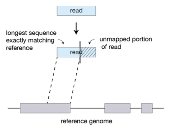
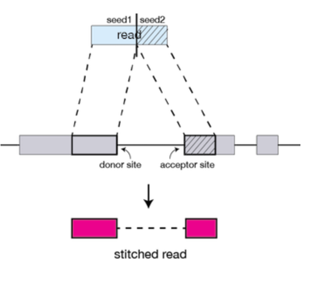
STAR searches for the longest sequence that exactly matches one or more locations on the reference genome. The longest match is called the Maximal Mappable Prefix (MMP).
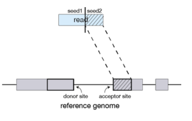
Portions of the read that are mapped separately are called ‘seeds’. So, the longest MMP for a read is called ‘seed1’.
Clustering, stitching, and scoring
In the second step of STAR, the separate seeds of a read are stitched together to create a complete read via clustering the seeds together based on proximity to a set of ‘anchor’ seeds (seeds that are not multi-mapping). Seeds are then stitched together based on the best alignment score for the read.
Figures from: https://hbctraining.github.io/Intro-to-rnaseq-hpc-O2/lessons/03_alignment.html
Reference Files for STAR
There are several reference files we will need to run STAR. Below we discuss the genome index and GTF file needed.
Genome Index
One important step that precedes running STAR for alignment is generation of a genome index. This step also uses the STAR module. A genome index takes the supplied reference genome sequences (FASTA files) and annotations (GTF file), generating a series of files that are used in the mapping step. Files included in this step include binary genome sequence, suffix arrays, text chromosome names/lengths, splice junctions coordinates, and transcripts/genes information. If you have to generate an index in the future, STAR strongly recommends not to change any of these files.
However, Biowulf conveniently provides users with a variety of reference data, including FASTA files, GTF files, and pre-built genome indices. For this reason, we will not be building an index today, but instead showing you how to access and use the resource already available on Biowulf.
This STAR data is available through the fdb directory. If you were with us back in session one, we mentioned the fdb directory on Biowulf, which is a shared data directory that houses a variety of genetics databases and reference data.
For our purposes today, we will use the path to the current STAR version data and the GENCODE reference information that we will be using:
/fdb/STAR_current/GENCODE/GENCODE_human/release_39
Release 39 of GENCODE is GRCh38, the genome build of our RNA-Seq data.
When it comes to choosing an index, these are named in accordance with the overhang, which is with respect to read length:
/fdb/STAR_current/GENCODE/Gencode_human/release_39/genes-###
‘###’ is the overhang value. Overhang is determined based on the Read length-1. You will see this when we run STAR later.
If you recall from the MultiQC report, both samples had a read length of 101 bp. Using the ReadLength -1 calculation, we will use the and genes-100 index to run the sample CS97520 through STAR.
/fdb/STAR_current/GENCODE/Gencode_human/release_39/genes-100
GTF File
The other file we will use is the GTF file, which contains gene and transcript coordinates. The path to this file is shown below:
/fdb/GENCODE/Gencode_human/release_39/gencode.v39.annotation.gtf
You will see the paths to both the genome indices and the GTF file in the swarm command used to run STAR.
Run STAR
Now we are ready to run STAR for sample CSP97520. Since this sample takes over one hour to run, we will set up a job, and then look at the expected results using pre-generated files.
1. To set up our job, we will use a sbatch command:
sbatch --cpus-per-task=12 --mem=100g scripts/session_10_star_align_FINAL.sh
We use the following arguments to set up our job:
- cpus-per-task - the number of CPUs to use for this job
- mem: the number of gigabytes of space needed
2. After running the command from step 2, you will see a job ID output. You can check the status of your job using various commands:
jobhist [jobID]
sjobs
squeue -u $USER
3. Now that we have our STAR job running, we can take a look at the sh script used to run STAR, session_10_star_align_FINAL.sh:
cat scripts/session_10_star_align_FINAL.sh
#!/usr/bin/env bash

GENOME_DIR=/fdb/STAR_current/GENCODE/Gencode_human/release_39/genes-100
THREADS=12
GTF_FILE=/fdb/GENCODE/Gencode_human/release_39/gencode.v39.annotation.gtf
OVERHANG=100
INPUT_DIR=/data/classes/DCEG_Somatic_Workshop/Practical_session_10/sample_data
FASTQ_1=CSP97520_1.fastq.gz
FASTQ_2=CSP97520_2.fastq.gz
SAMPLE=CSP97520
PLATFORM=ILLUMINA

module load STAR
module load samtools

mkdir ${SAMPLE}

cd ${SAMPLE}

STAR --twopassMode Basic \
        --genomeDir $GENOME_DIR \
        --runThreadN $THREADS \
        --outSAMtype BAM SortedByCoordinate \
        --sjdbGTFfile $GTF_FILE \
        --twopass1readsN -1 \
        --sjdbOverhang $OVERHANG \
        --readFilesIn $INPUT_DIR/$FASTQ_1 $INPUT_DIR/$FASTQ_2 \
        --readFilesCommand zcat \
        --quantMode TranscriptomeSAM GeneCounts \
        --outSAMattrRGline ID:$SAMPLE SM:$SAMPLE PL:$PLATFORM \
        --outFilterMultimapScoreRange 1 \
        --outFilterMultimapNmax 20 \
        --outFilterMismatchNmax 10 \
        --alignIntronMax 500000 \
        --alignMatesGapMax 1000000 \
        --sjdbScore 2 \
        --alignSJDBoverhangMin 1 \
  	   --outFilterMatchNminOverLread 0.33 \
        --outFilterScoreMinOverLread 0.33 \
        --outSAMattributes NH HI NM MD AS XS nM \
        --outSAMunmapped Within \
        --chimSegmentMin 12 \
        --chimJunctionOverhangMin 8 \
        --chimOutJunctionFormat 1 \
        --alignSJstitchMismatchNmax 5 -1 5 5 \
        --chimMultimapScoreRange 3 \
        --chimScoreJunctionNonGTAG -4 \
        --chimMultimapNmax 20 \
        --chimNonchimScoreDropMin 10 \
        --peOverlapNbasesMin 12 \
        --peOverlapMMp 0.1 \
        --alignInsertionFlush Right \
        --alignSplicedMateMapLminOverLmate 0 \
        --alignSplicedMateMapLmin 30 \
        --outFileNamePrefix ${SAMPLE}

samtools index ${SAMPLE}Aligned.sortedByCoord.out.bam
rm -r ${SAMPLE}_STARtmp
- Line 1: Set up our environment
- Line 3-11: Set up the variables to be used throughout the script
- Line 13 and 14: Load necessary modules
- Line 16: Create a directory for the STAR output
- Line 18: Move into that directory
- Lines 20-55: STAR command. Below you will find a description of each argument used.
- Line 57: Generate an index file to go with the BAM file (will be used later)
- Line 58: Remove the temporary folder STAR creates while running to store intermediate files
In lines 3-11, we set up the variables to be used throughout the script. Let’s look at a these lines to see what each of these is equivalent to:
GENOME_DIR=/fdb/STAR_current/GENCODE/Gencode_human/release_39/genes-100
THREADS=12
GTF_FILE=/fdb/GENCODE/Gencode_human/release_39/gencode.v39.annotation.gtf
OVERHANG=100
INPUT_DIR=/data/classes/DCEG_Somatic_Workshop/Practical_session_10/sample_data
FASTQ_1=CSP97520_1.fastq.gz
FASTQ_2=CSP97520_2.fastq.gz
SAMPLE=CSP97520
PLATFORM=ILLUMINA
| Variable Name | Description | Value |
|---|---|---|
| GENOME_DIR | Path to where genome indices are stored. | fdb/STAR_current/GENCODE/Gencode_human/release_39/genes-100 |
| THREADS | Number of threads to use to run STAR | 24 |
| GTF_FILE | Path to GTF file | /fdb/GENCODE/Gencode_human/release_39/gencode.v39.annotation.gtf |
| OVERHANG | Value to be used for sjdbOverhang argument | 100 |
| INPUT_DIR | Path to input data files | /data/classes/DCEG_Somatic_Workshop/Practical_session_10/sample_data |
| FASTQ_1 | Path to R1 fastq file | CSP97520_R1.fastq.gz |
| FASTQ_2 | Path to R2 fastq file | CSP97520_R2.fastq.gz |
| SAMPLE | Sample name (for RG line) | CSP97520 |
| PLATFORM | Platform name (for RG line) | ILLUMINA |
Below is a description of all of the different arguments being used in our STAR command:
twopassMode Basic: two-pass mapping mode. Here we use the Basic option for 2-pass mapping, meaning that the 1st pass of mapping is performed, then it will automatically extract junctions, insert them into the genome index, and, finally, re-map all reads in the 2nd mapping pass.genomeDir $GENOME_DIR: path to where the genome indices are storedrunThreadN 24: number of threads used for joboutSAMtype BAM SortedByCoordinate: generate output data files that are of BAM format and sortedsjdbGTFfile $GTF_FILE: specifies the path to the file with annotated transcripts in the standard GTF format. We use a file available on Biowulf, where we store the path to the file in the $GTF_FILE variable, as discussed above.twopass1readsN -1: number of reads to process for the 1st step. -1 means to map all reads in the first step.sjdbOverhang $OVERHANG: specifies the length of the genomic sequence around the annotated junction to be used in constructing the splice junctions database. Ideally, this length should be equal to the ReadLength-1, where ReadLength is the length of the reads. We also set this as a variable due to the samples having different ReadLengths.readFilesIn $FASTQ_1 $FASTQ_2: paths to the fastq files. Stored in variables as shown above.readFilesCommand zcat: un-compression commandquantMode TranscriptomeSAM GeneCounts:count number reads per gene while mapping. Here we will get both the Aligned.toTranscriptome.out.bam and ReadsPerGene.out.tab outputs.outSAMattrRGline ID:$SAMPLE SM:$SAMPLE PL:$PLATFORM: SAM/BAM read group line for easier identification of sample later on. Here we set it up to be the sample name and platform used.outFilterMultimapScoreRange 1: the score range below the maximum score for multimapping alignmentsoutFilterMultimapNmax 20:maximum number of loci the read is allowed to map to (i.e. multimapping reads)outFilterMismatchNmax 10: maximum number of mismatches per pairalignIntronMax 500000: maximum intron sizealignMatesGapMax 1000000: maximum gap between two matessjdbScore 2: extra alignment score for alignments that cross database junctionsalignSJDBoverhangMin 1: minimum overhang (i.e. block size) for annotated (sjdb) spliced alignmentsoutFilterMatchNminOverLread 0.33: alignment will be output only if the number of matched bases is higher than or equal to this value, normalized to read lengthoutFilterScoreMinOverLread 0.33:alignment will be output only if its score is higher than or equal to this value, normalized to read lengthoutSAMattributes NH HI NM MD AS XS nM: string of desired SAM attributes, in the order desired for the output SAM. Tags can be listed in any combination/order.NH*- number of loci the reads maps to: =1 for unique mappers, >1 for multimappers.HI*- multiple alignment index, starts with –outSAMattrIHstart (=1 by default).NM*- edit distance to the reference (number of mismatched + inserted + deleted bases) for each mate.MD*- string encoding mismatched and deleted reference bases (see standard SAM specifications)AS*- local alignment score, +1/-1 for matches/mismateches, score* penalties for indels and gaps. For PE reads, total score for two matesXS- alignment strandnM- number of mismatches. For PE reads, sum over two mates.
outSAMunmapped Within: output unmapped reads within the main alignment fileoutFileNamePrefix $SAMPLE: output files name prefix
The following arguments we included in our STAR command are specific to downstream analyses including fusion detection, splicing, etc.
chimSegmentMin 12: for the detection of chimeric (fusion) alignments; controls the minimum mapped length of the two segments that is allowedchimJunctionOverhangMin 8: minimum overhang for a chimeric junctionchimOutJunctionFormat 1: formatting type for the Chimeric.out.junction file; a 1 here means that the comment lines at the end of the file are command line andNreads: total, unique/multi-mappingalignSJstitchMismatchNmax 5 -1 5 5: maximum number of mismatches for stitching of the splice junctions; 1) non-canonical motifs, 2) GT/AC and CT/AC motif, 3) GC/AG and CT/GC motif, AT/AC, and GT/AT motifchimMultimapScoreRange 3: the score range for multi-mapping chimeras below the best chimeric scorechimScoreJunctionNonGTAG -4: penalty for a non-GT/AG chimeric junctionchimMultimapNmax 20: maximum number of chimeric multi-alignmentschimNonchimScoreDropMin 10: to trigger chimeric detection, the drop in the best non-chimeric alignment score with respect to the read length has to be greater than this valuepeOverlapNbasesMin 12: minimum number of overlap bases to trigger mates merging and realignment. Specify >0 value to switch on the “merging of overlapping mates” algorithmpeOverlapMMp 0.1: maximum proportion of mismatched bases in the overlap arealignInsertionFlush Right: how to flush ambiguous insertion positionsalignSplicedMateMapLminOverLmate 0: alignSplicedMateMapLmin 30: normalized to mate length
See the STAR manual for more information at this link.
STAR Output
You will see many output files when STAR has finished running. Below we explain what each of these files are using the CSP97520 example:
Files
- CSP97520Log.final.out- summary mapping statistics after mapping job is complete, very useful for quality control
- CSP97520Log.out- main log file with a lot of detailed information about the run. This file is most useful for troubleshooting and debugging
- CSP97520Log.progress.out- reports job progress statistics, such as the number of processed reads, % of mapped reads etc. It is updated in 1 minute intervals.
- CSP97520Aligned.sortedByCoord.out.bam- the genome-aligned BAM file for all sequencing reads
- CSP97520Aligned.sortedByCoord.out.bam.bai- index file for the BAM file, necessary for downstream analysis (ex. visualization)
- CSP97520Aligned.toTranscriptome.out.bam- alignments translated into transcript coordinates; will be used later for RSEM (transcript quantification)
- CSP97520ReadsPerGene.out.tab- read counts per gene with 4 columns which correspond to: 1) gene ID, 2) counts for unstranded RNA-seq, 3) counts for the 1st read strand aligned with RNA, and 4) counts for the 2nd read strand aligned with RNA
- CSP97520Chimeric.out.junction- contains detailed information in GTF format about chimerically-aligned reads; this file is important for use in downstream fusion analysis (only available with the additional arguments)
- CSP97520SJ.out.tab- contains splice junctions identified
Folders
- CSP97520_STARgenome- genome index
- CSP97520_STARpass1- first mapping pass information
Note: STAR also provides an option to retain temporary files or not.
In the next part of the practical session we go through post-alignment quality assessment, viewing one of the most important output files, the CSP97520Log.final.out file.
Post-alignment quality assessment
Next we are going to assess the quality of alignments in two ways, checking the STAR log file and applying PicardTools.
Quality assessment with STAR log files
If the STAR job completed successfully, you will find a file name with the extension Log.Final.out. This is a summary of the alignment statistics. We can open the file with the command:
cd /data/$USER/practical_session_10/STAR_output
cat CSP97520Log.final.out
You should see the following information.
                                 Started job on |       Apr 21 08:19:45
                             Started mapping on |       Apr 21 08:40:45
                                    Finished on |       Apr 21 09:19:07
       Mapping speed, Million of reads per hour |       113.48

                          Number of input reads |       72563351
                      Average input read length |       202
                                    UNIQUE READS:
                   Uniquely mapped reads number |       67560979
                        Uniquely mapped reads % |       93.11%
                          Average mapped length |       199.48
                       Number of splices: Total |       53113298
            Number of splices: Annotated (sjdb) |       53050512
                       Number of splices: GT/AG |       52553396
                       Number of splices: GC/AG |       439390
                       Number of splices: AT/AC |       51792
               Number of splices: Non-canonical |       68720
                      Mismatch rate per base, % |       0.54%
                         Deletion rate per base |       0.01%
                        Deletion average length |       1.32
                        Insertion rate per base |       0.01%
                       Insertion average length |       1.68
                             MULTI-MAPPING READS:
        Number of reads mapped to multiple loci |       3979660
             % of reads mapped to multiple loci |       5.48%
        Number of reads mapped to too many loci |       9523
             % of reads mapped to too many loci |       0.01%
                                  UNMAPPED READS:
  Number of reads unmapped: too many mismatches |       96903
       % of reads unmapped: too many mismatches |       0.13%
            Number of reads unmapped: too short |       876362
                 % of reads unmapped: too short |       1.21%
                Number of reads unmapped: other |       39924
                     % of reads unmapped: other |       0.06%
                                  CHIMERIC READS:
                       Number of chimeric reads |       350850
                            % of chimeric reads |       0.48%
Some statistics are good indicators of the alignment quality. Unique reads are reads with unambiguous mapping, which is typically highly quality alignments. So pay attention to the stats Uniquely mapped reads number and Uniquely mapped reads %.
In the category of MULTI-MAPPING READS, Number of reads mapped to multiple loci are reads mapped to more than one place, but less than the limit set in the STAR parameter(–outFilterMultimapNmax) , Number of reads mapped to too many loci are reads mapped to more than the limit.
CHIMERIC READS are counted as a separate category. It does not add up to the mapped or unmapped reads.
The STAR log file provides important but limited information. So usually we would want to use specific tools for a comprehensive post-alignment QC.
Quality assessment with Picard Tools
In the Picard Tools package, there are several tools for different types of QC. We would run two of them today. You could check the full list of the tools from here.
1. Let’s use the following script to submit the job.
cd /data/$USER/practical_session_10/scripts
swarm -t 2 -g 8 --time 4:00:00 --job-name qc post_alignment_qc.swarm
If we check the swarm file, we only process the sample CSP97520 using the bash file post_alignment_qc.sh. But we could process samples in batches in one job submission, and each sample/each swarm command line will run in parallel. Let’s review the bash file.
vi post_alignment_qc.sh

#/bin/bash
module load picard/2.25.0
module load R
REF_FLAT="/fdb/GATK_resource_bundle/hg38-v0/GRCh38_gencode.v27.refFlat.txt"
rRNA_list="/fdb/GATK_resource_bundle/hg38-v0/gencode.v27.rRNA.interval_list"

SAMPLE=$1
DIR=$2
mem=8g
thread=2

SECONDS=0
java -Xmx$mem -XX:ParallelGCThreads=$thread -jar $PICARDJARPATH/picard.jar CollectRnaSeqMetrics \
     -I $DIR/${SAMPLE}Aligned.sortedByCoord.out.bam \
     -O $DIR/Picard_RNA_Metrics.txt \
     --REF_FLAT $REF_FLAT \
     --STRAND NONE \
     --RIBOSOMAL_INTERVALS $rRNA_list
duration=$SECONDS
echo "CollectRnaSeqMetrics completed. $(($duration / 60)) minutes and $(($duration % 60)) seconds elapsed."

java -Xmx$mem -XX:ParallelGCThreads=$thread -jar $PICARDJARPATH/picard.jar CollectInsertSizeMetrics \
     -I $DIR/${SAMPLE}Aligned.sortedByCoord.out.bam \
     -O $DIR/insert_size_metrics.txt \
     -H $DIR/insert_size_histogram.pdf
duration=$SECONDS
echo "CollectInsertSizeMetrics completed. $(($duration / 60)) minutes and $(($duration % 60)) seconds elapsed."
In the lines beginning with java, you will find the names of the tools.
2. CollectRnaSeqMetrics produces RNA alignment metrics. For the full instruction of this tool, please refer to this link. Please note, in the picard tools website, the usage example looks like:
java -jar picard.jar CollectRnaSeqMetrics \
      I=input.bam \
      O=output.RNA_Metrics \
      REF_FLAT=ref_flat.txt \
      STRAND=SECOND_READ_TRANSCRIPTION_STRAND \
      RIBOSOMAL_INTERVALS=ribosomal.interval_list
The format I=input.bam is now replaced with -I input.bam in the latest version of picard tools, but the old format can also be recognized, with a warning message in output.
3. CollectInsertSizeMetrics is a tool to validate library construction and provides metrics of the insert size distribution and read orientation of paired-end libraries. For the full instruction of this tool, please refer to this link.
4. Now let’s check the output of the two files. We have included the output in the folder /data/$USER/practical_session_10/quality_checks. Open the output for CollectRnaSeqMetrics.
cd /data/$USER/practical_session_10/quality_checks
less Picard_RNA_Metrics.txt
In the header lines it contains the command and full set of options that generate the output file. The –INPUT and –OUTPUT could be different in the files you generated corresponding to your settings.
# CollectRnaSeqMetrics --REF_FLAT /fdb/GATK_resource_bundle/hg38-v0/GRCh38_gencode.v27.refFlat.txt --RIBOSOMAL_INTERVALS /fdb/GATK_resource_bundle/hg38-v0/gencode.v27.rRNA.interval_list --STRAND_SPECIFICITY NONE --INPUT /data/Sherlock_Lung/zhaow5/course/session10/STAR_output/CSP97520/CSP97520Aligned.sortedByCoord.out.bam --OUTPUT /data/Sherlock_Lung/zhaow5/course/session10/STAR_output/CSP97520/Picard_RNA_Metrics.txt --MINIMUM_LENGTH 500 --RRNA_FRAGMENT_PERCENTAGE 0.8 --METRIC_ACCUMULATION_LEVEL ALL_READS --ASSUME_SORTED true --STOP_AFTER 0 --VERBOSITY INFO --QUIET false --VALIDATION_STRINGENCY STRICT --COMPRESSION_LEVEL 5 --MAX_RECORDS_IN_RAM 500000 --CREATE_INDEX false --CREATE_MD5_FILE false --GA4GH_CLIENT_SECRETS client_secrets.json --help false --version false --showHidden false --USE_JDK_DEFLATER false --USE_JDK_INFLATER false
The main results is stored as a tab–delimited table (line 7-8)
PF_BASES        PF_ALIGNED_BASES        RIBOSOMAL_BASES CODING_BASES    UTR_BASES       INTRONIC_BASES  INTERGENIC_BASES        IGNORED_READS   CORRECT_STRAND_READS INCORRECT_STRAND_READS  NUM_R1_TRANSCRIPT_STRAND_READS  NUM_R2_TRANSCRIPT_STRAND_READS  NUM_UNEXPLAINED_READS   PCT_R1_TRANSCRIPT_STRAND_READS  PCT_R2_TRANSCRIPT_STRAND_READS       PCT_RIBOSOMAL_BASES     PCT_CODING_BASES        PCT_UTR_BASES   PCT_INTRONIC_BASES      PCT_INTERGENIC_BASES    PCT_MRNA_BASES       PCT_USABLE_BASES        PCT_CORRECT_STRAND_READS        MEDIAN_CV_COVERAGE      MEDIAN_5PRIME_BIAS      MEDIAN_3PRIME_BIAS      MEDIAN_5PRIME_TO_3PRIME_BIAS SAMPLE  LIBRARY READ_GROUP
14657796902     14260223050     7027    8881759830      4327050852      657672954       393732387       0       0       0       101036  51237144        607470       0.001968        0.998032        0       0.622835        0.303435        0.046119        0.027611        0.92627 0.901146        0       0.541722    0.557999 0.548583        0.896819
We can extract only the table (line 7-8) with this command
sed -n 7,8p Picard_RNA_Metrics.txt
-n suppresses the default output (that is, printing the whole file). 7,8p specifies the range of lines to extract. We can also write the table to a new file by redirecting the output:
sed -n 7,8p Picard_RNA_Metrics.txt >Picard_RNA_Metrics_table.txt
Now if we examine this table, unlike STAR log files that counts the number of reads, the Picard RNA metrics use nucleotide bases. PF_BASES are the number of bases in the PF reads, or reads that a filter of Illumina sequencer. The definition of all the metrics can be found here.
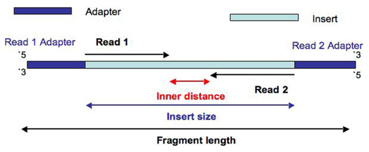
The insert size is illustrated as the diagram from a nice post https://www.biostars.org/p/106291/:
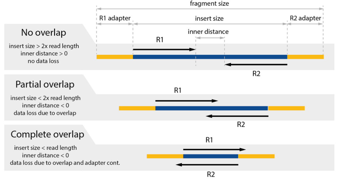
The overlap is observable if the insert size is lower than 2× the read length (see below). The shorter is the insert size, relative to the read length, the higher is the data loss. More information regarding the impact of insert size in RNA-seq could be found in this paper.
The output of CollectInsertSizeMetrics include a text file insert_size_metrics.txt and a pdf file insert_size_histogram.pdf.
5. We have included the Picard Tools results for the other example (CSP107316) in the folder Practical_session_10/quality_checks for comparison.
Visualization of alignment
Now can visualize the alignment results using IGV. We have used IGV to examining variants in practical session 4 (https://nci-iteb.github.io/tumor_epidemiology_approaches/sessions/session_4/practical#examining-variants-in-igv). You can follow the same steps to open the files.
Locate IGV on your computer and double click it to launch the application. In the upper left of the IGV window you will see a dropdown menu to select a reference genome. Select GRCh38/hg38.
Next you will need to load the BAM files into IGV. If you have mounted the biowulf account into your local laptop, then you can locate the files in the folder /data/$USER/practical_session_10/STAR_output. Alternatively click here to download them from GitHub.
Load them into IGV by clicking File » Load from File…, locating your downloaded files, and selecting CSP97520Aligned.sortedByCoord.out.bam.
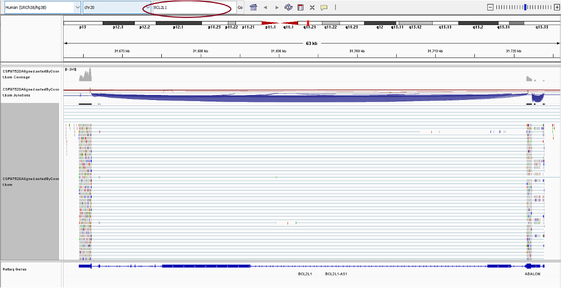
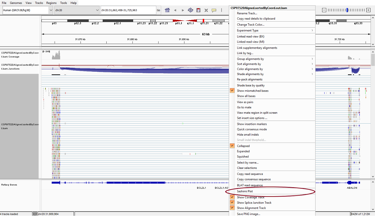
Next we would search for the gene BCL2L1. In the upper panel, you will see a search bar, in which you can enter ‘BCL2L1’. You should see this screen.
There are three tracks for each BAM file, from top to bottom:
Coverage Track to view depth of coverage
Splice Junction Track which provides an alternative view of reads spanning splice junctions
Alignment Track to view individual aligned reads
In the alignment track, you will see the pile–up view for all the reads mapping the region. You can right click the alignment track to change visualization options from the drop-down list.
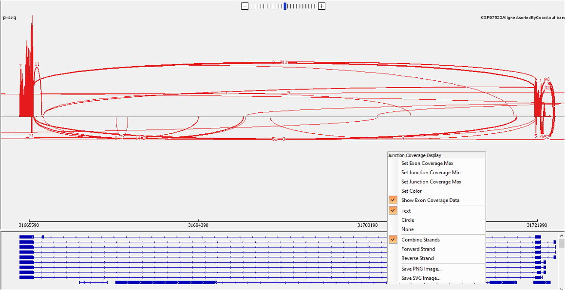
Next you could generate a sashimi plot to visualize the junction. In the drop-down list, select ‘Sashimi Plot’. To filter the junctions with low coverage, you could right click the top panel and select ‘Set Junction Coverage Min’ from the drop-down list.
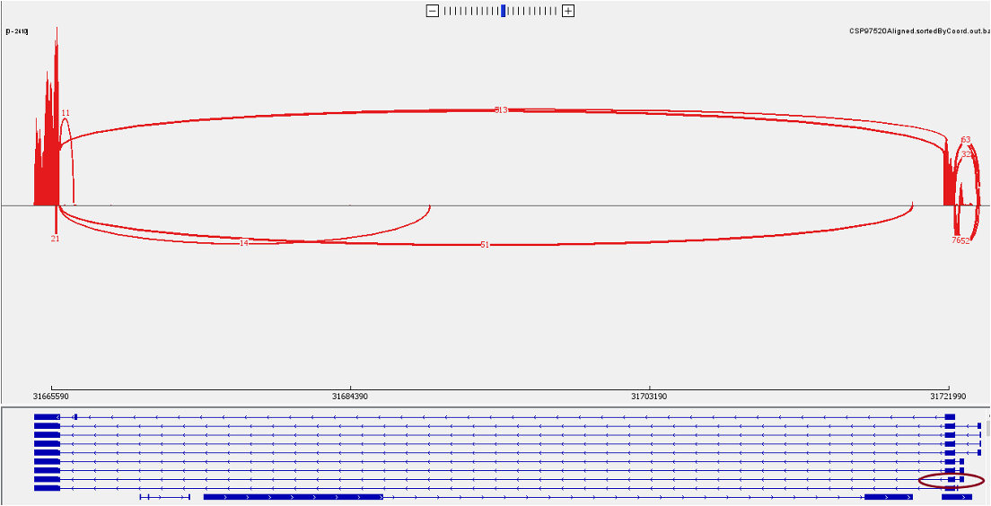
Now let’s look at the bottom panel. To see the detailed annotation, you could hover the mouse over the corresponding track. For BCL2L, there are two isoforms, the longer isoform BCL-X(L) and shorter isoform BCL-X(S). We can identify the short isoform from the exon highlighted below.
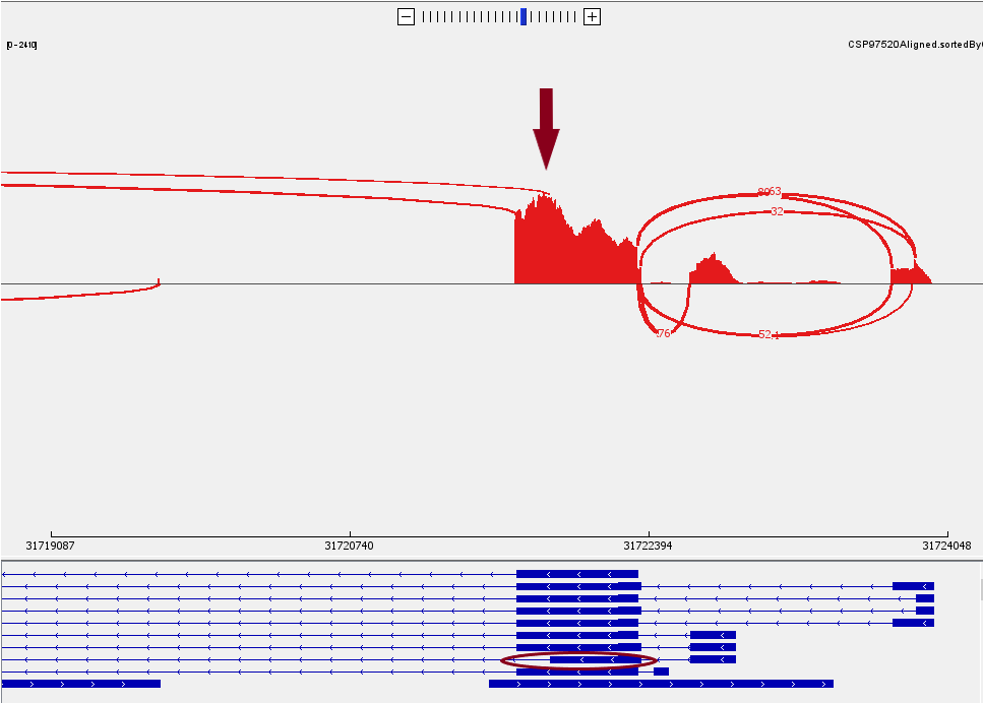
In a zoom-in view, we can identify the number of reads that support the junction of the short isoform BCL-X(S).
Gene/Transcript quantification using htseq and RSEM
Next we are going to show the gene quantification using two approaches, htseq and RSEM. In addition, when we run STAR with –quantMode GeneCounts option, STAR will count number reads per gene while mapping and output the result in file ReadsPerGene.out.tab.
Gene quantification using htseq
We have prepared a script to use htseq for quantification. Let’s first submit the commands.
cd ../scripts/
swarm -t 4 -g 8 --time 10:00:00 --job-name htseq htseq_quant.swarm
In the swarm file, you will find the bash file name htseq_quant.sh. Let’s check this file.
htseq-count  -m intersection-nonempty \
-i gene_id \
-r pos \
-s no
When counting the number of reads mapping to specific features, some reads are mapped to or overlap with more than one feature. For those reads, htseq-count allows the users to choose between three modes. Under the option -m, we can use union, intersection-strict or intersection-nonempty. For the difference between these modes, please refer to this link.
-i option specifies the attributes in GTF/GFF files to be used as the identifier of features.
-r options is how the alignment file is sorted. For paired-end data, the input alignment files have to be sorted either by read name or by alignment position, which can be done by samtools sort.
-s option is whether the data is from a strand-specific assay.
The output file (CSP97520_htseq.txt ) can be found in /data/$USER/practical_session_10/quantification.
Gene quantification using RSEM
Prepare RSEM reference files
For the first time we run RSEM, it is required to prepare transcript references for RSEM and optionally build BOWTIE/BOWTIE2/STAR/HISAT2 indices. We used the following scripts to generate the references. For the sake of time, we have included the references in the folder /data/classes/DCEG_Somatic_Workshop/Practical_session_10/ref/hg38_v39. So we skip this step for now.
As we would see shortly, we can use the BAM file generated by STAR for quantification. So it is important to ensure the consistency of all the reference files (.fasta file and .GTF file) between STAR and RSEM.
module load STAR/2.7.10b
module load rsem
fasta=/fdb/STAR_current/GENCODE/Gencode_human/release_39/ref.fa
GTF=/fdb/GENCODE/Gencode_human/release_39/gencode.v39.annotation.gtf
reference_name=/data/classes/DCEG_Somatic_Workshop/Practical_session_10/ref/hg38_v39

rsem-prepare-reference  --gtf $GTF \
--star \
$fasta \
$reference_name
Estimation of gene and transcript levels for individual sample
To apply RSEM to individual samples, we may use either the read sequence files (.fastq files) or the alignment files (.bam) files. Next we run the following commands to submit the swarm file:
swarm -t 4 -g 20 --time 8:00:00 --job-name rsem --gres=lscratch:100 rsem_from_bam.swarm
In the swarm file, you will find the bash file name rsem_from_bam.sh. Let’s get a look.
#!/bin/bash
module load rsem

reference_name=/data/classes/DCEG_Somatic_Workshop/Practical_session_10/ref/hg38_v39
SAMPLE=$1
DIR=$2
bam=$DIR/${SAMPLE}Aligned.toTranscriptome.out.bam
output_prefix=$DIR/$SAMPLE

rsem-calculate-expression -p $SLURM_CPUS_PER_TASK --temporary-folder /lscratch/$SLURM_JOBID/tempdir \
--paired-end \
--alignments \
--append-names \
$bam \
$reference_name $output_prefix
Break down of the arguments and options:
-p specifies the threads.
--alignments This argument specifies that the input file contains alignments in SAM/BAM/CRAM format. The exact file format will be determined automatically.
--append-names If gene_name/transcript_name is available, append it to the end of gene_id/transcript_id (separated by ‘_’) in files ‘sample_name.isoforms.results’ and ‘sample_name.genes.results’.
The argument $output_prefix will be used as the prefix of all output files (e.g., sample_name.genes.results).
Alternatively, RSEM can use .fastq files as input. In the pipeline that includes an alignment module, it is not necessary to re-do the alignment. It follows a different synopsis:
rsem-calculate-expression [options] --paired-end upstream_read_file(s) downstream_read_file(s) reference_name sample_name
Where upstream_read_file and downstream_read_file are fastq files of paired two reads respectively. When the input files are in fastq format, we can skip the –bam option and let RSEM generate an alignment file with the option –output-genome-bam. RSEM is compatible with multiple aligners, including Bowtie, Bowtie2, STAR and HISAT2. Here we use the option --star to specify STAR for the alignment.
Change to the practical_session_10 directory using cd ../ before we move on to the next part.
Review and compare the results of htseq and RSEM
The htseq generates one output file CSP97520_htseq.txt. It is a tab-delimited text file. You could check up with the command:
head -5 quantification/CSP97520_htseq.txt.
ENSG00000000003.15      2928
ENSG00000000005.6       0
ENSG00000000419.14      2022
ENSG00000000457.14      1001
ENSG00000000460.17      679
It has two columns. The first column is the gene id defined by the GTF file. The second column is the read counts.
The RSEM generates two output files with the extensions of rsem.genes.results and rsem.isoforms.results. We check the results with the command:
head -5 quantification/CSP97520.genes.results
gene_id transcript_id(s)        length  effective_length        expected_count  TPM     FPKM
ENSG00000000003.15_TSPAN6       ENST00000373020.9_TSPAN6-201,ENST00000494424.1_TSPAN6-202,ENST00000496771.5_TSPAN6-203,ENST00000612152.4_TSPAN6-204,ENST00000614008.4_TSPAN6-205     3520.94 3331.70 2747.00 14.63   13.73
ENSG00000000005.6_TNMD  ENST00000373031.5_TNMD-201,ENST00000485971.1_TNMD-202   873.50  684.29  0.00    0.00    0.00
ENSG00000000419.14_DPM1 ENST00000371582.8_DPM1-201,ENST00000371584.9_DPM1-202,ENST00000371588.10_DPM1-203,ENST00000413082.1_DPM1-204,ENST00000466152.5_DPM1-205,ENST00000494752.1_DPM1-206,ENST00000681979.1_DPM1-207,ENST00000682366.1_DPM1-208,ENST00000682713.1_DPM1-209,ENST00000682754.1_DPM1-210,ENST00000683010.1_DPM1-211,ENST00000683048.1_DPM1-212,ENST00000683466.1_DPM1-213,ENST00000684193.1_DPM1-214,ENST00000684628.1_DPM1-215,ENST00000684708.1_DPM1-216  1080.43 891.19       1884.28 37.51   35.21
ENSG00000000457.14_SCYL3        ENST00000367770.5_SCYL3-201,ENST00000367771.11_SCYL3-202,ENST00000367772.8_SCYL3-203,ENST00000423670.1_SCYL3-204,ENST00000470238.1_SCYL3-205 3154.92 2965.69 1002.28 6.00    5.63
The first line is the header. Each line is the statistics and quantification results for one gene. You may notice the length of genes may not be integer values. RSEM considers the length as abundance-weighted mean length of its isoforms. Length is this transcript’s sequence length (poly(A) tail is not counted). effective_length counts only the positions that can generate a valid fragment.
The expected_count in this file is equivalent to the read counts in the htseq output. But as we mentioned in the lecture, htseq and RSEM handle the multiple-mapped reads in different ways. RSEM ‘rescues’ the reads utilizing an Expectation-Maximization (EM) algorithm. So we would expect non-integer values in expected_count.
In addition to estimated raw counts, RSEM also provides two types of normalized counts, TPM and FPKM. A detailed introduction of these normalized quantification would be included in Lecture and Practical sessions for Session 11.
Lastly, let’s check the other output file of RSEM:
head -5 quantification/CSP97520.isoforms.results
transcript_id   gene_id length  effective_length        expected_count  TPM     FPKM    IsoPct
ENST00000373020.9_TSPAN6-201    ENSG00000000003.15_TSPAN6       3768    3578.77 2682.24 13.30   12.48   90.90
ENST00000494424.1_TSPAN6-202    ENSG00000000003.15_TSPAN6       820     630.77  0.00    0.00    0.00    0.00
ENST00000496771.5_TSPAN6-203    ENSG00000000003.15_TSPAN6       1025    835.77  62.07   1.32    1.24    9.01
ENST00000612152.4_TSPAN6-204    ENSG00000000003.15_TSPAN6       3796    3606.77 2.69    0.01    0.01    0.09
It is very similar to the gene-level results. But now the features being analyzed are transcript. And there is an additional column IsoPct, which is the percentage of this transcript’s abundance over its parent gene’s abundance.

