Presenters: Wei Zhao, Jian Sang, Alyssa Klein
Practical 4
Before we begin, please login to Biowulf and request an interactive session:
For a reminder on how to log-in to Biowulf, we refer you to this Biowulf HPC guide. In short:
- (Windows) use PuTTy
- (Mac) enter
ssh USERNAME@biowulf.nih.govto your terminal, then enter your password
Request an interactive session with the following command:
sinteractive --mem=12g --cpus-per-task=2
This practical section will focus on somatic mutational calling and downstream analysis. Today’s tasks include (A) performing somatic mutational calling using the GATK pipeline, (B) annotating the mutation calls, (C) visualizing somatic mutations in IGV, and (D) downstream analysis using MAFtools.
The GATK pipeline of somatic short variant (SNVs and indels) discovery
We will use the targeted sequencing data of paired tumor and normal samples from kidney for this practice. The scripts for this task will takes about 25 mins running time, so we will submit the scripts to Biowulf at the beginning of the session and then walk through the scripts together.
1. First let’s create a new folder in your personal data directory, and copy all the sample data to this directory.
cd /data/$USER/
mkdir practical_session_4
cd practical_session_4
cp -r /data/classes/DCEG_Somatic_Workshop/Practical_session_4/* .
2. Next, we will submit two sets of scripts to Biowulf. Use the following commands to submit the scripts for step 1.
cd shfiles
jobid1=$(swarm -t 8 -g 24  --gres=lscratch:24 --job-name step1 --time 1:00:00 scripts_for_step1.swarm)
echo $jobid1
swarm is a command to submit a group of command lines to biowulf and those command lines will run as parallel processes. The options -g, -t and –time specify the memory (in GB), threads and running time per process. We request 8CPUs and 24GB of memory for each process. The default running time is 2hrs. We assign a job name using the option –job-name. The option –gres is to allocate a local scratch disk space for each process. lscratch:N will require N GB for the scratch space. The directory of this scratch space can be accessed in the script as /lscratch/$SLURM_JOB_ID/. More information could be found at https://hpc.nih.gov/apps/swarm.html.
The swarm will return a job ID and it will be saved to $jobid1 in this script. We then submit the swarm file for step 2 and let it start only after the completion of all commands in the first job. To set up the dependency, we use the option –dependency=afterany:jobid where the jobid is $jobid1. Step 1 will take about 9 mins.
jobid2=$(swarm -t 8 -g 20 --gres=lscratch:20 --dependency=afterany:$jobid1 --job-name step2 scripts_for_step2.swarm)
echo $jobid2
In a few seconds, let’s check the job status using sjobs, the second job will sit in a pending state until all the processes in job1 are finished.
Data pre-processing for somatic short variant discovery
While we are waiting for the two jobs, let’s examine the script.
vi scripts_for_step1.swarm
#!/bin/bash
sh Step1_preprocess_variant_discovery.sh GPK7017_2000 ../fastq ../Results
sh Step1_preprocess_variant_discovery.sh GPK4013_0401 ../fastq ../Results
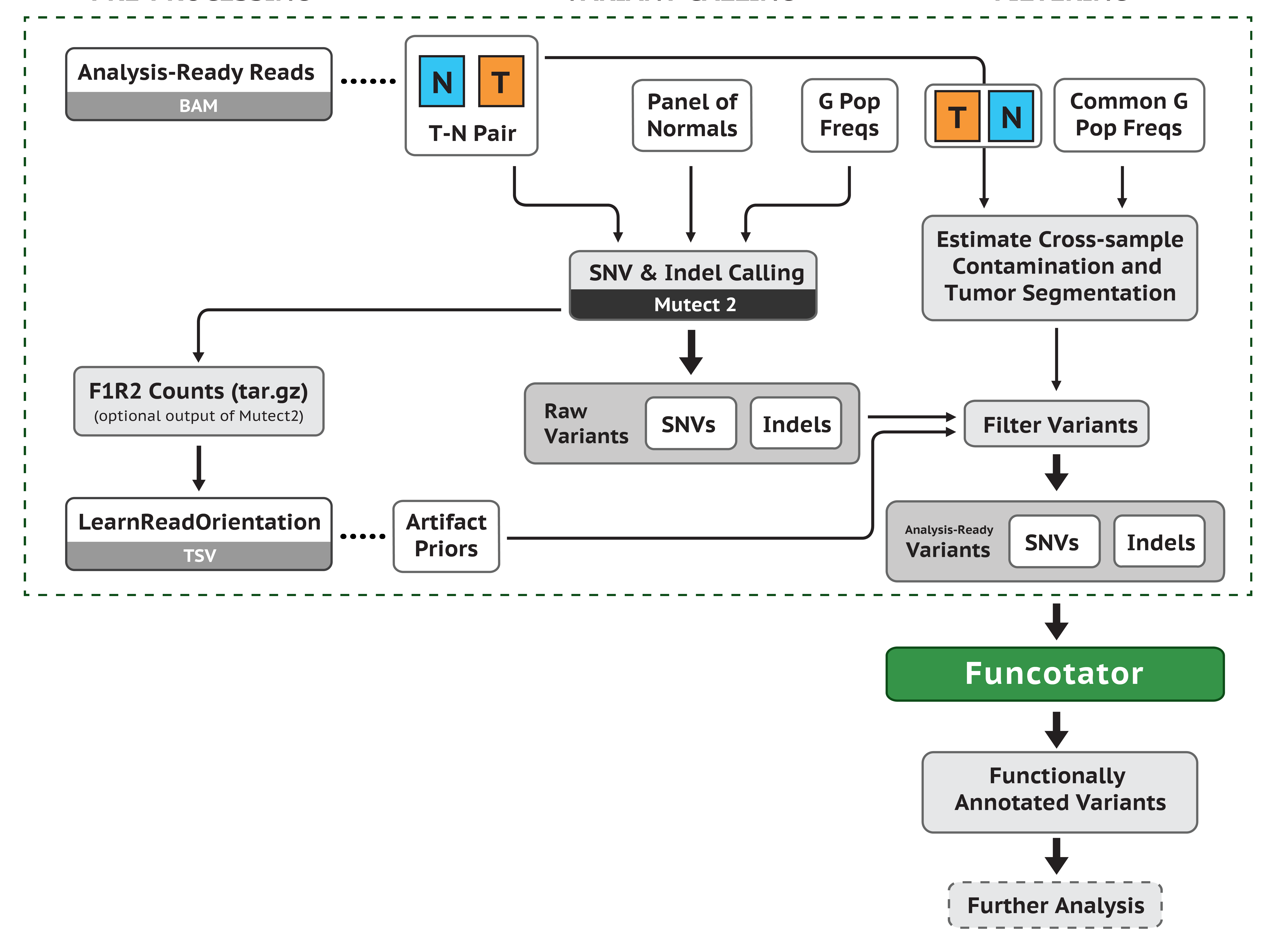
The first step for somatic or germline variant discovery is to pre-process the raw sequence data to produce analysis-ready BAM files. As the following figure shows, we start from the raw FASTQ files (or BAM files), align them to the reference genome, and clean up the data to correct for technical biases (e.g. duplicate reads, strand bias, cross-sample contamination, etc).

3. In the swarm file, each line corresponds to one sample, and will be submitted as one process in the swarm submission. They are all in the format:
sh ./Step1_preprocess_variant_discovery.sh $SAMPLE $INPUT_DIR $OUTPUT_DIR.
All the fields after the bash file (.sh) are arguments, and they will be passed to the bash (.sh) file. All the arguments in the swarm commands should be processed within the bash file. In this way, we can prepare the ‘core’ commands as bash files to process samples in batches.
4. Now let’s quit the swarm file by typing :q and hitting enter, and open the corresponding bash file.
vi Step1_preprocess_variant_discovery.sh
#!/bin/bash

#### Data preprocess for somatic short variant discovery using GATK workflow ###

module load samtools
module load bwa
module load fastp
module load GATK/4.3.0.0
module load picard/2.27.3

GATK_Bundle=/fdb/GATK_resource_bundle/hg38-v0
GENOME=$GATK_Bundle/Homo_sapiens_assembly38.fasta

SAMPLE=$1
INDIR=$2
DIR=$3
logs=$DIR/logs
read1=$INDIR/${SAMPLE}_R1.fastq.gz
read2=$INDIR/${SAMPLE}_R2.fastq.gz
id=$SAMPLE
lb=$id
sm=$id

SECONDS=0

echo -e "sample:$SAMPLE\nindir:$INDIR\noutdir:$DIR"

if [ ! -d "$DIR" ]; then
        mkdir -p $DIR
fi
if [ ! -d "$logs" ]; then
        mkdir -p $logs
fi
### Perform adaptor trimming on fastq files ###
fastp -i $read1 -I $read2 \
      --stdout --thread 2 \
      -j ${logs}/fastp-${SAMPLE}.json \
      -h ${logs}/fastp-${SAMPLE}.html \
      2> ${logs}/fastp-${SAMPLE}.log | \
bwa mem -M -t 8 \
      -R "@RG\tID:$id\tPL:ILLUMINA\tLB:$lb\tSM:$sm" \
      $GENOME - 2> ${logs}/bwa-${SAMPLE}.log | \
samtools sort -T /lscratch/$SLURM_JOB_ID/ -m 2G -@ 4 -O BAM \
      -o $DIR/${SAMPLE}_sort.bam  2> ${logs}/samtools-${SAMPLE}.log

###/lscratch/$SLURM_JOBID
duration=$SECONDS
echo "Alignment completed. $(($duration / 60)) minutes and $(($duration % 60)) seconds elapsed."

### Duplicate marking in coordinate-sorted raw BAM files ###
java -Xmx2g -jar $PICARDJARPATH/picard.jar MarkDuplicates \
     -I $DIR/${SAMPLE}_sort.bam \
    -O /dev/stdout \
    -M marked_dup_metrics.txt 2> ${logs}/markdup-${SAMPLE}.log \
|java -Xmx2g -jar $PICARDJARPATH/picard.jar SortSam \
      -I /dev/stdin -O $DIR/${SAMPLE}_markdup_sorted.bam \
      -SORT_ORDER coordinate 2>> ${logs}/markdup-${SAMPLE}.log

duration=$SECONDS
echo "Duplicate marking completed. $(($duration / 60)) minutes and $(($duration % 60)) seconds elapsed."

DBSNP=/fdb/GATK_resource_bundle/hg38/dbsnp_138.hg38.vcf.gz
INDEL=/fdb/GATK_resource_bundle/hg38-v0/Homo_sapiens_assembly38.known_indels.vcf.gz
GOLD_INDEL=/fdb/GATK_resource_bundle/hg38-v0/Mills_and_1000G_gold_standard.indels.hg38.vcf.gz

### Recaliberating base quality score###
gatk --java-options "-Djava.io.tmpdir=/lscratch/$SLURM_JOBID -Xms6G -Xmx6G -XX:ParallelGCThreads=2" BaseRecalibrator \
  -I $DIR/${SAMPLE}_markdup_sorted.bam \
  -R $GENOME \
  -O  $DIR/${SAMPLE}_markdup_bqsr.report \
  --known-sites $DBSNP \
  --known-sites $INDEL \
  --known-sites $GOLD_INDEL \
  > ${logs}/BQSR-${SAMPLE}.log 2>&1

gatk --java-options "-Djava.io.tmpdir=/lscratch/$SLURM_JOBID -Xms6G -Xmx6G -XX:ParallelGCThreads=2" ApplyBQSR \
  -I $DIR/${SAMPLE}_markdup_sorted.bam  \
  -R $GENOME \
  --bqsr-recal-file  $DIR/${SAMPLE}_markdup_bqsr.report \
  -O  $DIR/${SAMPLE}_markdup_bqsr.bam \
  >> ${logs}/BQSR-${SAMPLE}.log 2>&1

duration=$SECONDS
echo "Base recaliration completed. $(($duration / 60)) minutes and $(($duration % 60)) seconds elapsed."
We first load several modules using module load. Then we specify the reference/source files to be used. Most of the reference files corresponding to a pre-installed application in Biowulf can be found in the folder /fdb/. Note the way we pass the arguments to the bash file. Arguments passed to a script are processed in the same order in which they’re sent (in this case, the order in the swarm file). The indexing of the arguments starts at one, and the first argument can be accessed inside the script using $1. Similarly, the second argument can be accessed using $2, and so on. Here we assign the first argument to variable $SAMPLE, and so on.
GATK_Bundle=/fdb/GATK_resource_bundle/hg38-v0
GENOME=$GATK_Bundle/Homo_sapiens_assembly38.fasta

SAMPLE=$1
INDIR=$2
DIR=$3
logs=$DIR/logs
read1=$INDIR/${SAMPLE}_R1.fastq.gz
read2=$INDIR/${SAMPLE}_R2.fastq.gz
id=$SAMPLE
lb=$id
sm=$id
5. We use the fastp command to trim the adapters, bwa to perform raw alignment to the reference genome, and samtools sort to sort the files by genomic coordinates. The three commands are connected by ‘pipes’ | to bypass storage of large intermediate files. The adapter trimming step is optional. The backslash at the end of each line is used to skip the line breaker and the command continues in the next line.
### Perform adaptor trimming on fastq files ###
fastp -i $read1 -I $read2 \
      --stdout --thread 2 \
      -j ${logs}/fastp-${SAMPLE}.json \
      -h ${logs}/fastp-${SAMPLE}.html \
      2> ${logs}/fastp-${SAMPLE}.log | \
bwa mem -M -t 8 \
      -R "@RG\tID:$id\tPL:ILLUMINA\tLB:$lb\tSM:$sm" \
      $GENOME - 2> ${logs}/bwa-${SAMPLE}.log | \
samtools sort -T /lscratch/$SLURM_JOB_ID/ -m 2G -@ 4 -O BAM \
      -o $DIR/${SAMPLE}_sort.bam  2> ${logs}/samtools-${SAMPLE}.log
Let’s take a look at the three commands separately:
In the last line of the fastp command lines, ‘2’ is a file descriptor. It redirects(writes) any ‘standard error’ messages to the log file fastp-${SAMPLE}.log, which will be otherwise output to the screen. In bwa mem options, -tspecifies the number of threads. -R specifies the read header lines. - indicates taking the input from the standard input. In this example, we used the pipes to redirect the standard output of last command (aka, fastp) as the standard input into the next command (bwa). So we use this option to tell the script take the output from command as the input data. In samtools sort options, -T is the prefix of temporary files. -m and -@ specify the memory per thread and the number of threads, respectively. -O specifies the output format.
6. Now we have a sorted raw alignment BAM file. In the next section of the script, we mark read pairs that are likely to have originated from duplicates of the same DNA fragments uing picard tools.
### Duplicate marking in coordinate-sorted raw BAM files ###
java -Xmx2g -jar $PICARDJARPATH/picard.jar MarkDuplicates \
     -I $DIR/${SAMPLE}_sort.bam \
    -O /dev/stdout \
    -M marked_dup_metrics.txt 2> ${logs}/markdup-${SAMPLE}.log \
| java -Xmx2g -jar $PICARDJARPATH/picard.jar SortSam \
      -I /dev/stdin -O $DIR/${SAMPLE}_markdup_sorted.bam \
      -SORT_ORDER coordinate 2>> ${logs}/markdup-${SAMPLE}.log
The picard tools package contains multiple commands, and the command lines look like this:
java [java opts] -jar $PICARDJARPATH/picard.jar COMMAND [options]
We use a pipe to connect two picard commands MarkDuplicates and SortSam. Similar to the bwa example, in the second picard command, we use -I /dev/stdin to specify reading from standard input.
7. In the last part of the script, we recalibrate base quality score to correct for patterns of systematic errors using the GATK tools for BQSR. The GATK command lines look like this:
gatk --java-options "[java opts]" ToolName [options]
### Recaliberating base quality score###
gatk --java-options "-Djava.io.tmpdir=/lscratch/$SLURM_JOBID -Xms6G -Xmx6G -XX:ParallelGCThreads=2" BaseRecalibrator \
  -I $DIR/${SAMPLE}_markdup_sorted.bam \
  -R $GENOME \
  -O  $DIR/${SAMPLE}_markdup_bqsr.report \
  --known-sites $DBSNP \
  --known-sites $INDEL \
  --known-sites $GOLD_INDEL \
  > ${logs}/BQSR-${SAMPLE}.log 2>&1

gatk --java-options "-Djava.io.tmpdir=/lscratch/$SLURM_JOBID -Xms6G -Xmx6G -XX:ParallelGCThreads=2" ApplyBQSR \
  -I $DIR/${SAMPLE}_markdup_sorted.bam  \
  -R $GENOME \
  --bqsr-recal-file  $DIR/${SAMPLE}_markdup_bqsr.report \
  -O  $DIR/${SAMPLE}_markdup_bqsr.bam \
  >> ${logs}/BQSR-${SAMPLE}.log 2>&1
The first tool BaseRecalibrator builds the recalibration model. As we calculate the mismatched bases, we exclude the loci known to vary in the population, which requires the input of known variants resource. And this is specified by the option –known-sites. The second tool, ApplyBQSR ,adjusts the score based on the model.
The command line > ${logs}/BQSR-${SAMPLE}.log 2>&1 redirects ‘standard error’ messages - denoted by file descriptor ‘2’ - to the ‘standard output’ - denoted by file descriptor ‘1’, and writes both mesagges to the log file BQSR-${SAMPLE}.log, which will be otherwise output to the screen.
8. By the end of step 1, you should have generated analysis-ready BAM files for each individual sample (tumor and normal). We prepared the sample output data in the /Results/ directory for you to check.
ls ../Expected_Results
Somatic short variant discovery using MuTect2
Next we will use the analysis-ready BAM files to proceed the GATK pipeline for somatic short variant discovery. There are two main steps: generating candidate variants and filtering. We use GATK tools for both steps. For more details please refer to: https://gatk.broadinstitute.org/hc/en-us/articles/360035894731-Somatic-short-variant-discovery-SNVs-Indels-.
Let’s examine the swarm file.
vi scripts_for_step2.swarm
#!/bin/bash
sh Step2_somatic_variant_discovery_MuTect2.sh  GPK7017_2000 GPK4013_0401 PAP1_1708_01_T01 ../Results ../Results
Simlar to the first step, we use one bash file to process tumor/normal sample pairs in batches. In this example, we have only one tumor/normal pair, but we can easily scale up in this way. Now let’s quit the swarm file by with :q and open the script file:
vi Step2_somatic_variant_discovery_MuTect2.sh
#!/bin/bash

#### Call somatic short variant discovery using MuTect2 and filtering ###

module load samtools
module load bwa
module load fastp
module load GATK/4.3.0.0
module load picard/2.27.3

GATK_Bundle=/fdb/GATK_resource_bundle/hg38-v0
GENOME=$GATK_Bundle/Homo_sapiens_assembly38.fasta
COMMONVAR=/data/classes/DCEG_Somatic_Workshop/Practical_session_4/Reference/small_exac_common_3.hg38.vcf.gz

NSAMPLE=$1
TSAMPLE=$2
PREFIX=$3
INDIR=$4
DIR=$5
logs=$DIR/logs

BAM_NORMAL=$INDIR/${NSAMPLE}_markdup_bqsr.bam
BAM_TUMOR=$INDIR/${TSAMPLE}_markdup_bqsr.bam
BASE_TUMOR=`samtools view -H $BAM_TUMOR |awk '$1~/^@RG/ {for (i=1;i<=NF;i++) {if ($i~/SM/) {split($i,aa,":"); print aa[2]}}}'|sort|uniq`
BASE_NORMAL=`samtools view -H $BAM_NORMAL | awk '$1~/^@RG/ {for (i=1;i<=NF;i++) {if ($i~/SM/) {split($i,aa,":"); print aa[2]}}}'|sort|uniq`

OUT_VCF=$DIR/${PREFIX}.vcf
OUT_FILTERED_VCF=$DIR/${PREFIX}_filtered.vcf
OUT_PASSED_VCF=$DIR/${PREFIX}_passed.vcf
OUT_STATS=$DIR/${PREFIX}.vcf.stats

SECONDS=0

if [ ! -d "$DIR" ]; then
        mkdir -p $DIR
fi
if [ ! -d "$logs" ]; then
        mkdir -p $logs
fi
### SNV and Indel calling  ###
gatk --java-options "-Djava.io.tmpdir=/lscratch/$SLURM_JOBID -Xms20G -Xmx20G -XX:ParallelGCThreads=1" Mutect2 \
  -R $GENOME \
  -I $BAM_NORMAL \
  -I $BAM_TUMOR \
  -normal $BASE_NORMAL \
  -tumor $BASE_TUMOR \
  -O $OUT_VCF \
  > ${logs}/Mutect2-${PREFIX}.log 2>&1

duration=$SECONDS
echo "MuTect2 completed. $(($duration / 60)) minutes and $(($duration % 60)) seconds elapsed."

### Filtering the MuTect2 variant calls ###
### Estimate cross-sample contamination  ###

gatk --java-options "-Xms10G -Xmx10G -XX:ParallelGCThreads=2" GetPileupSummaries \
   -I $BAM_TUMOR \
   -V $COMMONVAR \
   -L $COMMONVAR \
   -O $DIR/${TSAMPLE}_pileups.table \
   > ${logs}/VarFilter-${PREFIX}.log 2>&1

gatk --java-options "-Xms10G -Xmx10G -XX:ParallelGCThreads=2" GetPileupSummaries \
   -I $BAM_NORMAL \
   -V $COMMONVAR \
   -L $COMMONVAR \
   -O $DIR/${NSAMPLE}_pileups.table \
   >> ${logs}/VarFilter-${PREFIX}.log 2>&1

gatk --java-options "-Xms10G -Xmx10G -XX:ParallelGCThreads=2" CalculateContamination \
     -I $DIR/${TSAMPLE}_pileups.table \
     -matched $DIR/${NSAMPLE}_pileups.table \
     -tumor-segmentation $DIR/${TSAMPLE}_segments.table \
     -O $DIR/${TSAMPLE}_calculatecontamination.table \
     >> ${logs}/VarFilter-${PREFIX}.log 2>&1

### Filter variants  ###

gatk --java-options "-Djava.io.tmpdir=/lscratch/$SLURM_JOBID -Xms20G -Xmx20G -XX:ParallelGCThreads=2" FilterMutectCalls \
  -R $GENOME \
  --contamination-table $DIR/${TSAMPLE}_calculatecontamination.table \
  --stats $OUT_STATS \
  --tumor-segmentation $DIR/${TSAMPLE}_segments.table \
  -O $OUT_FILTERED_VCF \
  -V $OUT_VCF \
  >> ${logs}/VarFilter-${PREFIX}.log 2>&1
awk '($1 ~/^#/) || ($7 ~ /PASS/) {print}' $OUT_FILTERED_VCF >$OUT_PASSED_VCF

###/lscratch/$SLURM_JOBID
duration=$SECONDS
echo "Filtering completed. $(($duration / 60)) minutes and $(($duration % 60)) seconds elapsed."
9. In the first part, we load necessary modules, specify reference resources and arguments from input. We pass five arguments from the swarm commands in the following order: normal sample name, tumor sample name, prefix for output file name (e.g. patient or subject ID), input file directory, and output file directory.
GATK_Bundle=/fdb/GATK_resource_bundle/hg38-v0
GENOME=$GATK_Bundle/Homo_sapiens_assembly38.fasta
COMMONVAR=/data/classes/DCEG_Somatic_Workshop/Practical_session_4/Reference/small_exac_common_3.hg38.vcf.gz

NSAMPLE=$1
TSAMPLE=$2
PREFIX=$3
INDIR=$4
DIR=$5
logs=$DIR/logs
10. In the next part, we use the GATK tool Mutect2 to call candidate variants.
### SNV and Indel calling  ###
gatk --java-options "-Djava.io.tmpdir=/lscratch/$SLURM_JOBID -Xms20G -Xmx20G -XX:ParallelGCThreads=1" Mutect2 \
  -R $GENOME \
  -I $BAM_NORMAL \
  -I $BAM_TUMOR \
  -normal $BASE_NORMAL \
  -tumor $BASE_TUMOR \
  -O $OUT_VCF \
  > ${logs}/Mutect2-${PREFIX}.log 2>&1
The options -I were used twice to specify the input BAM files for normal and tumor samples, respectively. The names of the tumor and normal samples are specified by the options -tumor and -normal, which have to match the sample names in the read group lines of the BAM file. Note that the read group lines take this format: @RG\tID:$id\tPL:ILLUMINA\tLB:$lb\tSM:$sm, and the sample names are in the last field.
If we are working with whole exome or genome sequencing data, then this step requires a large amount of memory. They can be changed in the java options -Xms and -Xmx. MuTect2 does not allow multithreading in its options. So to spped up this process, you may consider parallel computing using a ‘scatter-gather’ approach, that is, run separate GATK commands to process a proportion of the input data and collate all the results into the final output. For more information, please refer to https://gatk.broadinstitute.org/hc/en-us/articles/360035532012-Parallelism-Multithreading-Scatter-Gather.
11. The next part of the script calculates the cross-sample contamination and estimates the allelic copy number segmentation for each tumor sample. It will generate a contamination-table file that will be used for filtering This is an optional step.
### Filtering the MuTect2 variant calls ###
### Estimate cross-sample contamination  ###

gatk --java-options "-Xms10G -Xmx10G -XX:ParallelGCThreads=2" GetPileupSummaries \
   -I $BAM_TUMOR \
   -V $COMMONVAR \
   -L $COMMONVAR \
   -O $DIR/${TSAMPLE}_pileups.table \
   > ${logs}/VarFilter-${PREFIX}.log 2>&1

gatk --java-options "-Xms10G -Xmx10G -XX:ParallelGCThreads=2" GetPileupSummaries \
   -I $BAM_NORMAL \
   -V $COMMONVAR \
   -L $COMMONVAR \
   -O $DIR/${NSAMPLE}_pileups.table \
   >> ${logs}/VarFilter-${PREFIX}.log 2>&1

gatk --java-options "-Xms10G -Xmx10G -XX:ParallelGCThreads=2" CalculateContamination \
     -I $DIR/${TSAMPLE}_pileups.table \
     -matched $DIR/${NSAMPLE}_pileups.table \
     -tumor-segmentation $DIR/${TSAMPLE}_segments.table \
     -O $DIR/${TSAMPLE}_calculatecontamination.table \
     >> ${logs}/VarFilter-${PREFIX}.log 2>&1
The tool GetPileupSummaries summarizes read counts that support reference, alternative and other alleles for given sites. In its options -V and -L, it requires an input file for common germline variant sites, e.g. this file from the gnomAD resource. We provide a reference file small_exac_common_3.hg38.vcf.gz in our folder. Other reference files for this purpose (e.g. gnomAD) can be found at the GATK Google bucket.
For your future reference: you may use the following commands within an interactive session to check and download the reference files for common germline variant sites (for today’s ).
module load google-cloud-sdk
gsutil ls gs://gatk-best-practices/somatic-hg38/
gsutil ls gs://gatk-best-practices/somatic-hg38/af-only-gnomad.hg38.vcf.gz* ./
12. Then we will filter the mutation candidates using the tool FilterMutationCalls. The options –contamination-table and –tumor-segmentation use the output from the previous step and are optional.
### Filter variants  ###

gatk --java-options "-Djava.io.tmpdir=/lscratch/$SLURM_JOBID -Xms20G -Xmx20G -XX:ParallelGCThreads=2" FilterMutectCalls \
  -R $GENOME \
  --contamination-table $DIR/${TSAMPLE}_calculatecontamination.table \
  --stats $OUT_STATS \
  --tumor-segmentation $DIR/${TSAMPLE}_segments.table \
  -O $OUT_FILTERED_VCF \
  -V $OUT_VCF \
  >> ${logs}/VarFilter-${PREFIX}.log 2>&1
awk '($1 ~/^#/) || ($7 ~ /PASS/) {print}' $OUT_FILTERED_VCF >$OUT_PASSED_VCF
This process annotates the variants as ‘PASS’ in the ‘FILTER’ field in its output VCF file, but will keep all the candidate variants, including those that failed the filtering, in its output. So we use an awk command to extract all the variants that pass the filtering.
13. At the end of step 2, we have VCF files for original candidates and candidates that pass the filtering. How do we check the number of candidate mutations in each file? We use these commands.
cd ../Expected_Results/
grep -v "^#" PAP1_1708_01_T01.vcf | wc -l
grep -v "^#" PAP1_1708_01_T01_passed.vcf | wc -l
grep -v will extract all lines that do NOT contain a specific pattern. The pattern we specify is “^#”, which is lines starting with the “#” symbol. This will exclude all the header lines in the VCF file. Then we redirect the output to the command wc -l which calculates the number of lines.
Annotation of somatic short variants
Now we have a list of variants ready for the downstream analysis. To prioritize the variants for downstream analysis. we will functionally annotate these variants. There are multiple applications for this analysis, and we are going to show two methods, Funcotator and ANNOVAR.
14. We first annotate with Funcotator. Confirm that you are in the interactive session, and enter the following commands.
cd /data/$USER/practical_session_4/shfiles
sh ./Step3_funcotator_annotation.sh  PAP1_1708_01_T01 ../Expected_Results ../Results
The script will take a few seconds. Let’s first check the bash scripts.
vi /data/classes/DCEG_Somatic_Workshop/Practical_session_4/shfiles/Step3_funcotator_annotation.sh
#!/bin/bash

#### Annotate VCF file with Funcotator ###

module load samtools
module load GATK/4.3.0.0

GATK_Bundle=/fdb/GATK_resource_bundle/hg38-v0
GENOME=$GATK_Bundle/Homo_sapiens_assembly38.fasta
FUNCOTATORDB=/fdb/GATK_resource_bundle/funcotator/funcotator_dataSources.v1.7.20200521s

PREFIX=$1
INDIR=$2
DIR=$3
logs=$DIR/logs
IN_VCF=$INDIR/${PREFIX}_passed.vcf
OUT_ANNOT_MAF=$DIR/${PREFIX}_funcotator.maf

if [ ! -d "$DIR" ]; then
        mkdir -p $DIR
fi
if [ ! -d "$logs" ]; then
        mkdir -p $logs
fi

SECONDS=0

gatk --java-options "-Xms10G -Xmx10G -XX:ParallelGCThreads=2" Funcotator -R $GENOME \
     -V $IN_VCF \
     -O $OUT_ANNOT_MAF \
     --output-file-format MAF \
     --data-sources-path $FUNCOTATORDB \
     --ref-version hg38

duration=$SECONDS
echo "Annotation completed. $(($duration / 60)) minutes and $(($duration % 60)) seconds elapsed."
Funcotator is a tool in the GATK package. It requires five input files:
-RA reference genome sequence.-VA VCF of variant calls to annotate.--data-sources-pathThe path to data sources or required formats.--ref_versionThe version of the reference genome sequence being used.--output-file-formatThe desired output format for the annotated variants file (MAF or VCF). We also specify the output file name with the -O option.
gatk --java-options "-Xms10G -Xmx10G -XX:ParallelGCThreads=2" Funcotator -R $GENOME \
     -V $IN_VCF \
     -O $OUT_ANNOT_MAF \
     --output-file-format MAF \
     --data-sources-path $FUNCOTATORDB \
     --ref-version hg38
All the data source files have already been downloaded in the Biowulf, so we specify the data source folder using this command:
FUNCOTATORDB=/fdb/GATK_resource_bundle/funcotator/funcotator_dataSources.v1.7.20200521s
The script takes three arguments to generate the input/output paths and file names: the prefix of the input VCF file, the input and output directories.
The basic output files in VCF or MAF format contains all variants from the input file, with added annotation from the data sources.
We will run the second annotation package ANNOVAR and check the results together later.
15. Next we annotate with ANNOVAR. The command lines are very similar:
cd /data/$USER/practical_session_4/shfiles
sh ./Step3_annovar_annotation.sh  PAP1_1708_01_T01 ../Expected_Results ../Results
Next let’s check the bash scripts.
vi /data/classes/DCEG_Somatic_Workshop/Practical_session_4/shfiles/Step3_annovarannotation.sh
#!/bin/bash

#### Annotate VCF file with ANNOVAR ###
module load annovar/2020-06-08

PREFIX=$1
INDIR=$2
DIR=$3
logs=$DIR/logs
IN_VCF=$INDIR/${PREFIX}_passed.vcf

if [ ! -d "$DIR" ]; then
        mkdir -p $DIR
fi
if [ ! -d "$logs" ]; then
        mkdir -p $logs
fi

echo $IN_VCF
echo $INDIR
echo $DIR
SECONDS=0

cd $DIR
convert2annovar.pl -format vcf4 $IN_VCF -includeinfo >${PREFIX}.avinput
table_annovar.pl  ${PREFIX}.avinput $ANNOVAR_DATA/hg38 \
	-buildver hg38 -out ${PREFIX} -remove \
	-protocol refGene,cytoBand,exac03,avsnp147,dbnsfp30a -operation g,r,f,f,f \
	-nastring . -csvout -polish

duration=$SECONDS
echo "Annotation completed. $(($duration / 60)) minutes and $(($duration % 60)) seconds elapsed."
The program convert2annovar.pl converts the VCF format into the ANNOVAR input format (.avinput file). For specification of the ANNOVAR input format, you may get more details at: https://annovar.openbioinformatics.org/en/latest/user-guide/input/.
convert2annovar.pl -format vcf4 $IN_VCF -includeinfo >${PREFIX}.avinput
table_annovar.pl  ${PREFIX}.avinput $ANNOVAR_DATA/hg38 \
	-buildver hg38 -out ${PREFIX} -remove \
	-protocol refGene,cytoBand,exac03,avsnp147,dbnsfp30a -operation g,r,f,f,f \
	-nastring . -csvout -polish
The program table_annovar.pl is the core command for annotation. -protocol specifies the annotation sources to use:ExAC version 0.3 (referred as exac03), dbNFSP version 3.0a (referred to as dbnsfp30a), dbSNP version 147 with left-normalization (referred to as avsnp147). Each ‘protocol’ corresponds to one field in the -option argument: gene-based (referred to as g), gene-based with cross-reference annotation (referred to as gx), region-based (referred to as r) and filter-based (referred to as f). In the final output file, a tab-delimited file with many columns will contain the input columns and annotation columns, that correspond to the combination of ‘protocol’ and ‘option’. For more details, please refer to https://annovar.openbioinformatics.org/en/latest/user-guide/startup/#table_annovarpl.
16. Now open the two output files for both software in Excel (you can right click » Save as… these links).
The Funcotator output is in the MAF format, the first several columns are the basic features of the mutation: genomic coordinates, reference and variant alleles, variant classifications and types. The variant classifications and types could be used to prioritize candidate driver mutations.

If we scroll to the right, there are annotations of genomic, cDNA and protein changes.

The ANNOVAR output is in VCF format. The first several columns include basic information about the variants. The columns of ‘Func.refGene’ and ‘ExonicFunc.refGene’ could be used to prioritize candidate driver mutations. The column ‘AAChange.refGene’ provides similar information to the protein changes annotated by Funcotator.

For the next a few columns, the ExAC* columns are allele frequencies in all the samples and the subpopulations in the Exome Aggregation Consortium data sets. The column ‘avsnp147’ is the SNP ID in the dbSNP database. The other columns are prediction scores for the likelihood of non-synonymous variants to be deleterious using several popular tools, such as SIFT, PolyPhen2, HDIV, LRT, and so on.

Examining variants in IGV
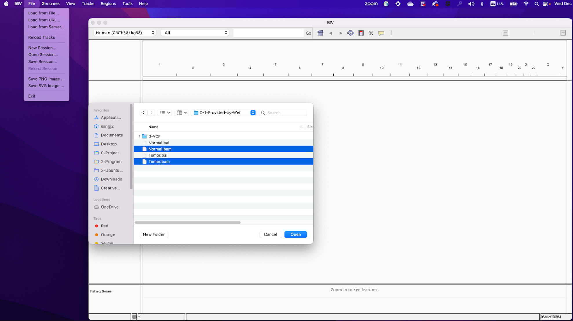
17. Locate IGV on your computer and double click it to launch the application.
18. In the upper left of the IGV window you will see a dropdown menu to select a reference genome. Select GRCh38/hg38.
19. Now you will need to load the BAM files into IGV. Click here to download them from GitHub (you may need to unzip the folder).
Once the files are downloaded, load them into IGV by clicking File » Load from File…, locating your downloaded files, and selecting Normal.bam and Tumor.bam.
20. You should see the loaded file names Normal.bam and Tumor.bam on the left side of the IGV window, which in IGV are referred to as ‘tracks’. In addition, you might also see “Normal.bam Junctions” and “Tumor.bam Junctions”. If you do, you can remove them by right clicking on these tracks and on the menu that appears click “Remove Track”. These junction tracks are not useful for today’s demonstration and will use extra computer memory, causing IGV to slow down.

Passing Variants
21.a. Now let’s examine some variants. First, search chr7:116782048
in the search bar at the top of the IGV window (boxed in red in the example image below). Individually right click “Normal.bam” and “Tumor.bam” and select Color alignments by » read strand in the menu that appears for each; this will allow you to clearly see which reads are forward-strand reads and which are reverse-strand reads.
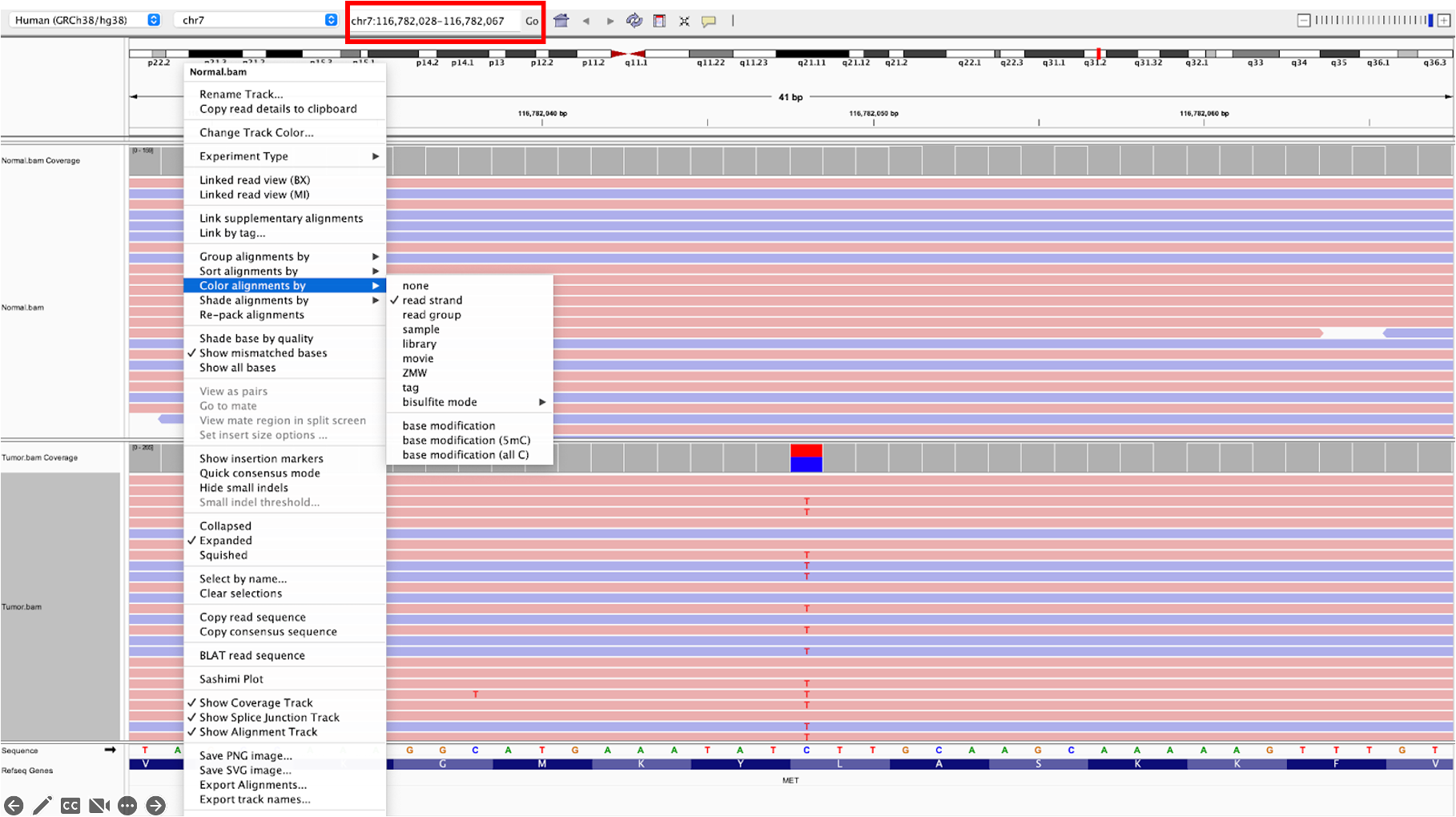
This variant is within an exon of the MET gene, and passes variant filters (FILTER column=”PASS” in the .vcf file).
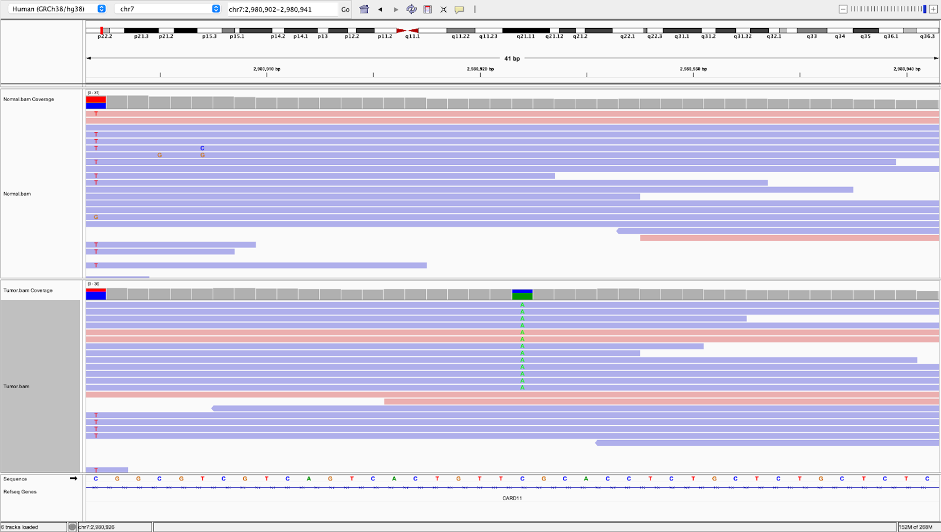
21.b. Likewise we can examine a passing intronic variant. In the search bar at the top, search for chr7:2980922
and hit Go.
Filtered Variants
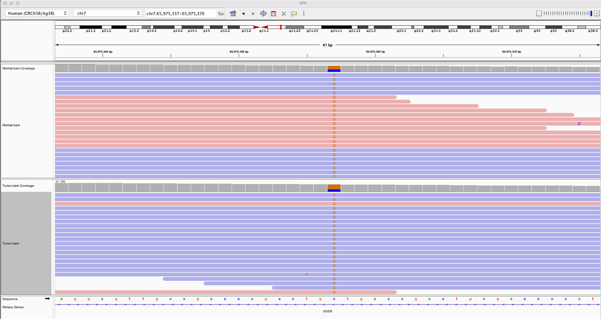
22.a. Let’s now examine some variants that do not pass filters. In the search bar at the top, search for chr7:65975357
. This variant was filtered because it was flagged as germline, and you can see that both the tumor and normal samples contain a roughly equal proportion of reads with a C>G variant.
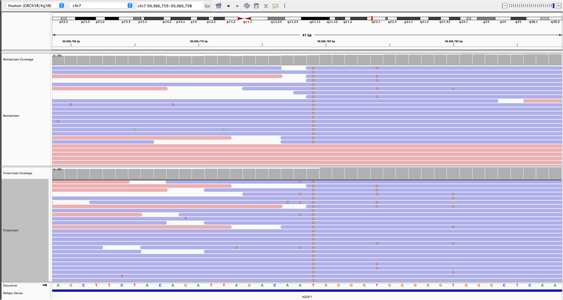
22.b. To see a variant exhibiting strand bias, search for chr7:99966779
in the search bar. As you can see, these variants are only detected on reverse-strand reads and not forward-strand reads, which is a likely sign of an artifact from sequencing.
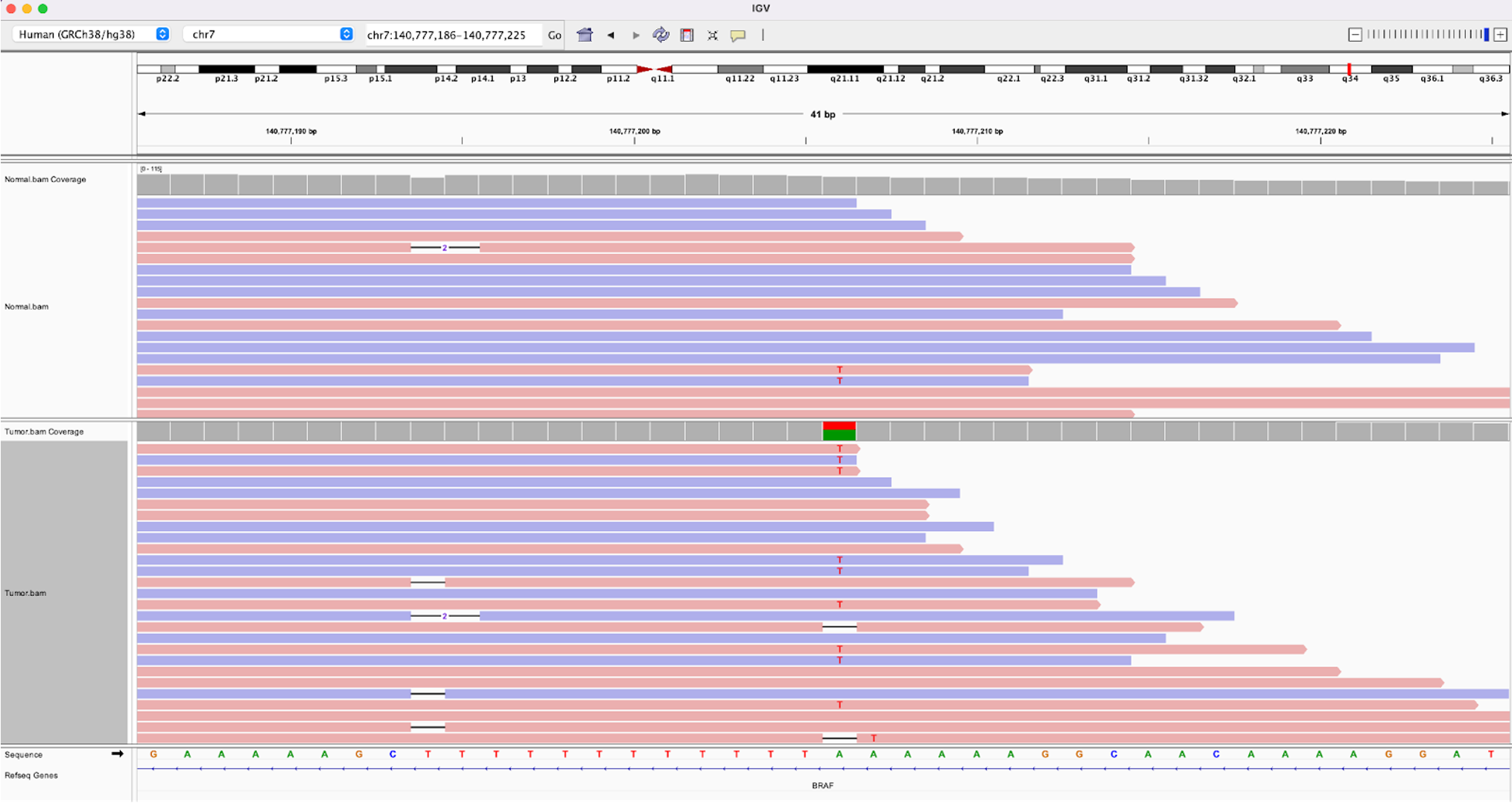
22.c. Lastly, we highlight a multi-allelic site. Search for chr7:140777206
. Here you can see at that genomic location the reference is an A, the tumor contains many A>T mutations, but also has several reads with a deletion at that location. Multi-allelic sites are generally very rare and are more likely to be a sign of a noisy region in the genome than a true variant.
Introduction to maftools
maftools is an R package designed to summarize, analyze, annotate, and visualize Mutation Annotation Format (MAF) files. Today, we will be using the maftools package to analyze and visualize the data within a MAF file.
The package consists of visualization and analysis based modules. The diagram below provides a visual representation of these modules as well as the inputs needed to run them.
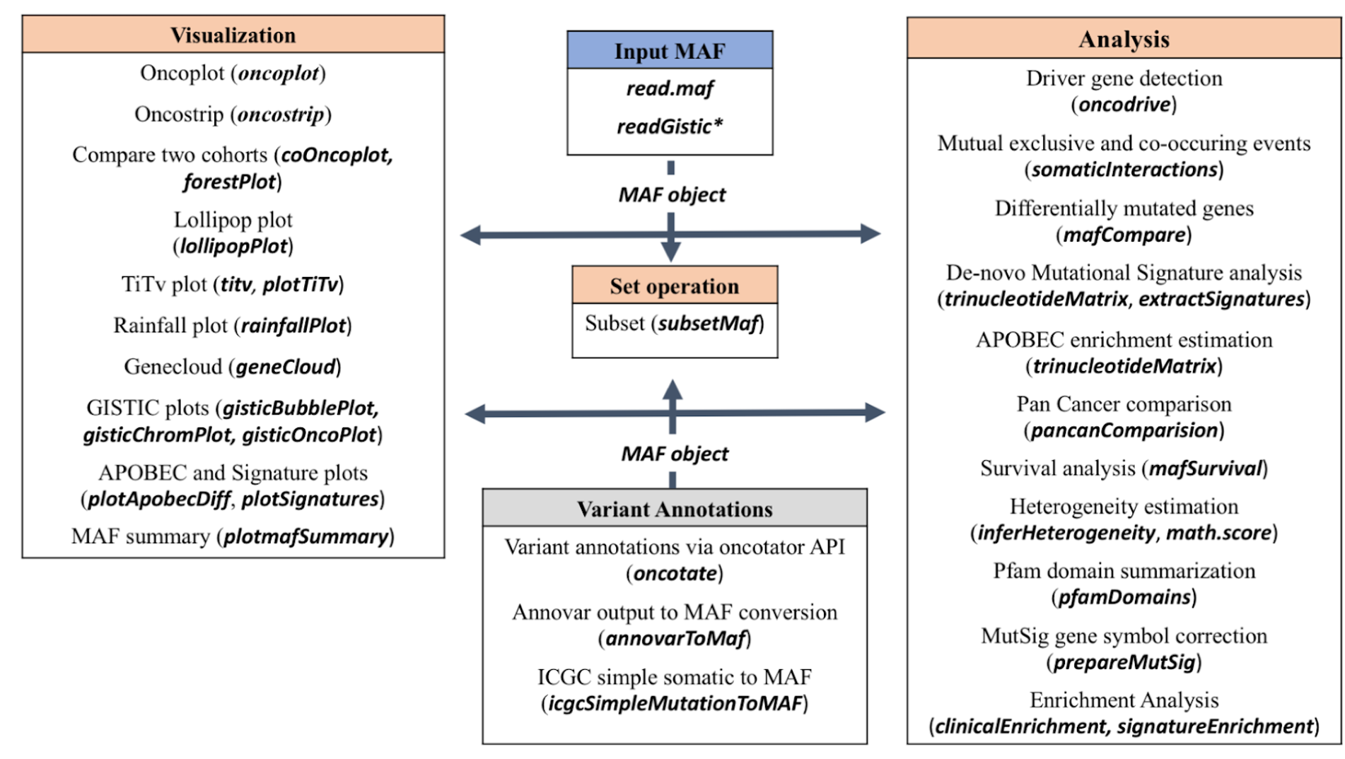
For a more in-depth explanation of maftools, how to use it, and its capabilities beyond our demonstration today, use this link.
Download session directory
23. First we will download the directory we have created for this session. This directory is called session4_maftools, and you can download it here. You may have to unzip the download first before use.
This directory includes 2 files: 1) the MAF data we will be using today, and 2) the R script with all of the commands you will find throughout this part of the practical session.
For consistency, move this downloaded directory to your Downloads folder.
Go to the session4_maftools folder and open the file, maf_session4_practice_FINAL.R.
Install and load maftools package in R
24. If you haven’t done so already, you will need to install the maftools package in R. Use the following commands to do this:
# install BiocManager if not already installed
if (!require("BiocManager"))
  install.packages("BiocManager")
# install maftools if not already installed
BiocManager::install("maftools")
The code above installs BiocManager if it is not already installed, and then uses BiocManager to install the maftools package. BiocManager is a package manager for the Bioconductor repository, which includes a series of R packages used for genomic analysis. Click these links for additional information about BiocManager or Bioconductor.
After you install maftools, load the package using the command:
library(maftools)
Additional Information: For some functions in exercises not being demonstrated today but available as supplemental information, you will need to use the tidyverse package.
Install the tidyverse package if you do not already have it installed. Then load tidyverse. This package contains a group of R packages that are useful for data analyses and visualization.
if(!('tidyverse' %in% installed.packages())){
  install.packages('tidyverse')
  library(tidyverse)
}else{
  library(tidyverse)
}
Load the data into R
25. Run getwd() to make sure that the current working directory (the computer folder R is working in) is the path to the session4_maftools folder:
>getwd()

Mac:
[1] "/Users/[username]/Downloads/session4_maftools"
Windows:
[1] "C:/Users/[username]/Downloads/session4_maftools"
If the working directory is not the session4_maftools directory, use the setwd() command to set this directory as the working directory (replace [username] with your NIH username):
Mac: setwd("/Users/[username]/Downloads/session4_maftools")
Windows: setwd("C:/Users/[username]/Downloads/session4_maftools")
Then run getwd() as before to make sure the working directory is now correct.
26. We have extracted over 550 TCGA-LUAD (lung adenocarcinoma) whole exome sequencing (WES) samples using the public MAF file generated as a part of the TCGA MC3 project. A sample manifest file was used to extract data for primary tumor WES samples from the public MAF file.
To load the MAF file, we will need to use the path to the file so it can be loaded into R. Use the command below to load the data file:
tcga_luad_maf <- read.maf(maf='tcga_luad_maf_final.gz')
You will see the following appear as the file is read, validated, and summarized:
-Reading
|--------------------------------------------------|
|==================================================|
-Validating
--Removed 17797 duplicated variants
-Silent variants: 70411
-Summarizing
--Possible FLAGS among top ten genes:
  TTN
  MUC16
  USH2A
-Processing clinical data
--Missing clinical data
-Finished in 14.2s elapsed (12.8s cpu)
Summarize the mutation data
27. For a quick summary of the maf object you have generated from the data loaded, simply type the object name. You will see a summary of the object.
tcga_luad_maf
An object of class MAF
                        ID summary    Mean Median
 1:             NCBI_Build  GRCh37      NA     NA
 2:                 Center       .      NA     NA
 3:                Samples     567      NA     NA
 4:                 nGenes   17339      NA     NA
 5:        Frame_Shift_Del    3986   7.030      5
 6:        Frame_Shift_Ins    1183   2.086      1
 7:           In_Frame_Del     387   0.683      0
 8:           In_Frame_Ins      37   0.065      0
 9:      Missense_Mutation  134468 237.157    164
10:      Nonsense_Mutation   11158  19.679     12
11:       Nonstop_Mutation     180   0.317      0
12:            Splice_Site    4517   7.966      5
13: Translation_Start_Site     224   0.395      0
14:                  total  156140 275.379    187
The summary of the object above shows you the genome build used in generating this data, the number of samples included, the number of genes included, and a variety of variant classification types, ranging from frame shifts to nonstop mutations.
Additional Information
You can generate a sample summary, a gene summary, explore the fields in the file (i.e. column names), and even write a MAF summary.
To generate a summary of the MAF file by sample:
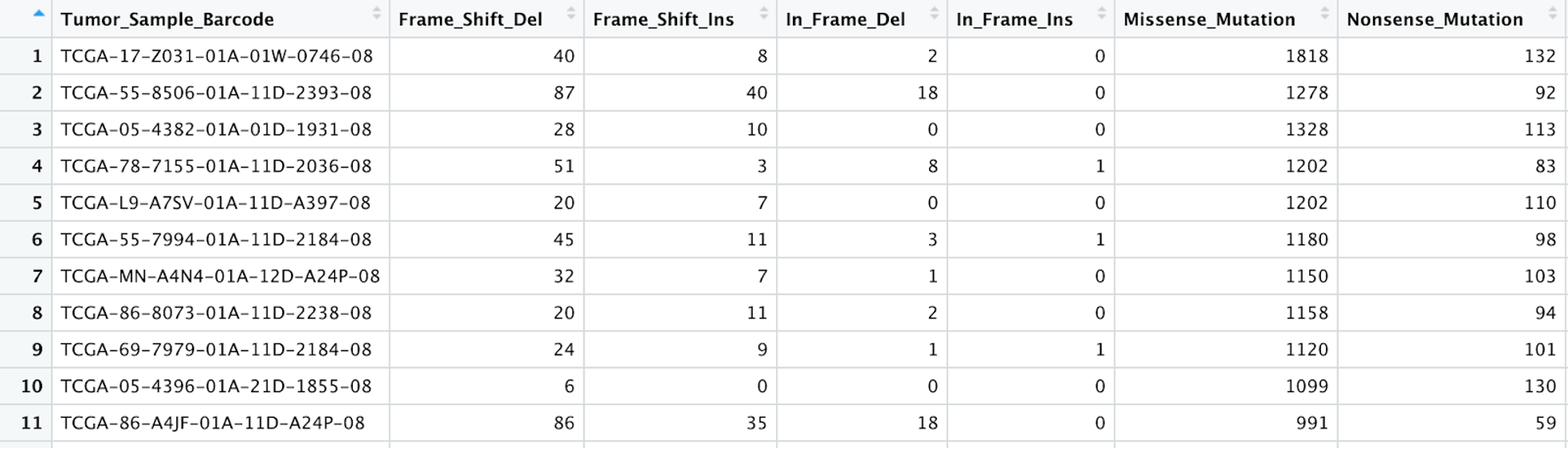
getSampleSummary(tcga_luad_maf)%>%View().Here is an example of what the first few rows and columns of that table look like:
To generate a summary of the MAF file by gene:
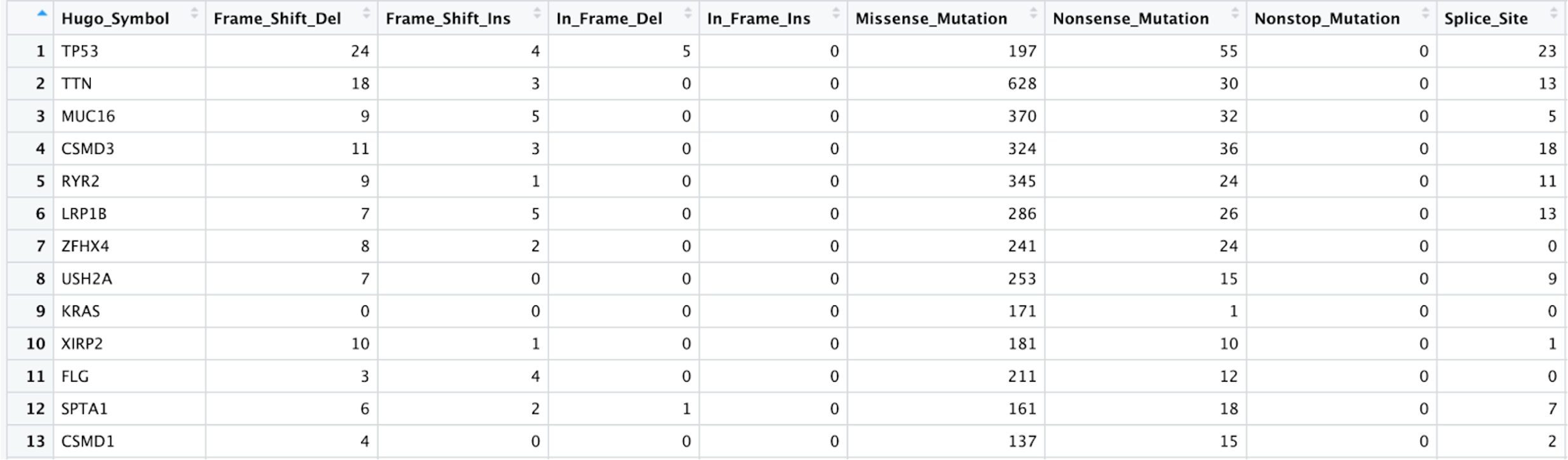
getGeneSummary(tcga_luad_maf)%>%View().Here is an example of what the first few rows and columns of that table look like:
Tip: Using View() opens them in a new tab in RStudio in an interactive table format. Otherwise the table will print directly to the R console in a format that is difficult to read.
getFields(tcga_luad_maf)This will print fields included in the MAF object. There are 114 fields in our object, so shown here are just the first 10.
[1] "Hugo_Symbol"                   "Entrez_Gene_Id"
[3] "Center"                        "NCBI_Build"
[5] "Chromosome"                    "Start_Position"
[7] "End_Position"                  "Strand"
[9] "Variant_Classification"        "Variant_Type"
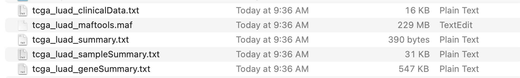
write.mafSummary(maf=tcga_luad_maf, basename='tcga_luad')This will save a MAF summary to your current working directory. This consists of several files, including clinicalData (if available), maftools.MAF, summary, sampleSummary, and geneSummary files. Here is an example of these files on a local machine after they have been generated:
Visualization and analysis with maftools
We are going to be running several analyses and generating several visualizations of the MAF data that you have successfully loaded into R.
plotmafSummary()
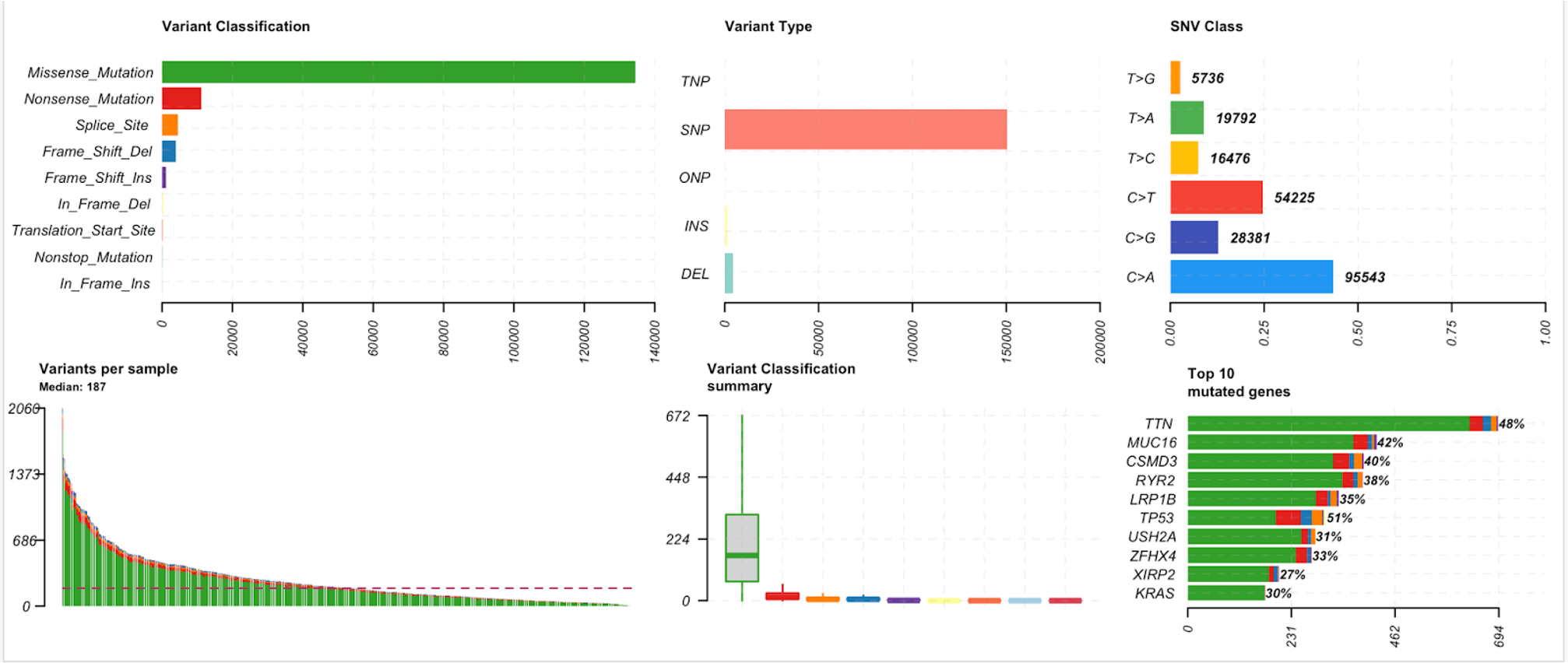
28. We will start with generating a plot of the MAF summary. This summary of the data includes variant classification, variant type, SNV class, variants per sample, a variant classification summary, and the top 10 mutated genes.
Use the following command to generate the MAF summary for the TCGA-LUAD data:
plotmafSummary(maf = tcga_luad_maf, rmOutlier = TRUE, addStat = 'median', dashboard = TRUE, titvRaw = FALSE)
Note: Additional parameters in this command include the following:
rmOutlier, which removes outliers from the boxplot if TRUEaddStat, adds median or mean to Variant per sample plot when set, otherwise set to NULLdashboard, plot dashboard instead of simple summary when TRUEtitvRaw, plots raw variant counts when FALSE or fractions when TRUE
Tip: For help as to how a function works or what additional arguments there are, you can use ?{function_name}. For example, ?plotmafSummary would provide information about this plotting function.
Below is a brief explanation for each of the components in the summary above
| Component | Description | Sample Interpretation |
|---|---|---|
Variant Classification 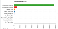 |
Total number of mutations for each variant classification category across all samples. | The TCGA-LUAD samples contain the most missense mutations over any other variant classification type. |
Variant Type  |
Total number of mutations for each variant type across all samples in a file. (SNP- Single Nucleotide Polymorphisms, TNP- Triple Nucleotide Polymorphism, ONP- Oligonucleotide Polymorphism, INS- insertion, DEL- deletion). For more information click here. | The TCGA-LUAD samples contain the greatest number of SNPs compared to any other variant type. |
SNV Class 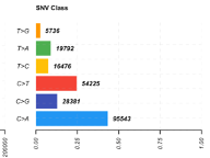 |
Total number of mutations for each Single Nucleotide Variant (SNV) class. There are six main SNV classes, as listed here: T>G, T>A, T>C, C>T, C>G, and C>A. The first base notes the original, and the base following the ‘>’ symbol is the mutated base. | In the TCGA-LUAD samples, there are almost 100,000 C>A mutations, which make up almost half of all of the SNVs in this TCGA-LUAD cohort. |
Variants per sample 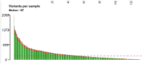 |
In this bar plot, samples are along the x-axis, and the total number of mutations in each sample are along the y-axis. These counts are colored by variant classification. The median number of variants per sample is shown as a dashed line. | In this TCGA-LUAD cohort, there are a median of 187 variants per sample. |
Variant Classification summary 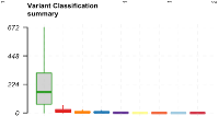 |
This plot is made up of a series of box plots, one for each variant classification category. It summarizes the median number of a given variant classification type across all samples. | The TCGA-LUAD samples contain the most missense mutations over any other variant classification type. The median number of missense mutations is close to 200. |
Top 10 mutated genes 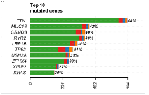 |
The bar plot shows the top 10 mutated genes in the cohort. The x-axis notes the number of variants per gene, and the y-axis contains the genes. The bars on the plot are colored by variant classification category. At the end of each bar there is a percentage, denoting the percentage of samples with at least one variant in the gene. | In the TCGA-LUAD samples, TTN was the most mutated gene, with almost 700 mutations in 48% of samples. TP53 was mutated in 51% of the samples, with about 250 mutations. |
oncoplot()
29.Now we will generate two different oncoplots for several different genes included in the MAF file. Oncoplots can help to visualize the mutational landscape of samples in a study or cohort.
First, we will generate an oncoplot for the top 10 most mutated genes in the TCGA-LUAD samples. Use the following command:
oncoplot(maf = tcga_luad_maf, top = 10)

The oncoplot shows the tumor mutational burden in each sample (top panel), the number of samples with a mutation in the given gene (right panel), and the variant classifications in each sample per gene (main panel). Each row is a gene and each column is a sample.
In the title of the plot, we can see that almost 90% of these samples have mutations in at least one of these top 10 genes. TP53 is mutated in the largest percentage of samples, 51%. We can also see that missense mutations are the dominant variant classification across these genes in the TCGA-LUAD samples.
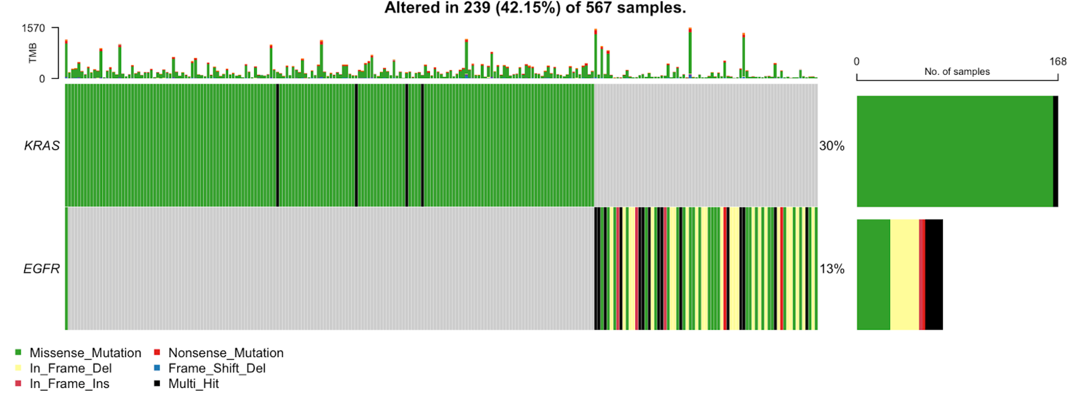
30. We can also generate an oncoplot for specific genes. See the example below where we plot only TP53, KRAS, and EGFR.
oncoplot(maf = tcga_luad_maf, genes = c('TP53','KRAS','EGFR'))
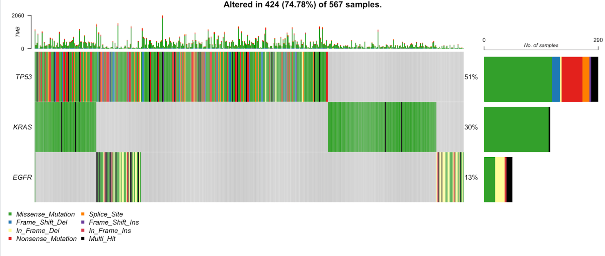
We see the TP53 and KRAS are similar to the first oncoplot, but it is evident that the samples along the x-axis are in a different order, due to the difference seen in the KRAS plot in the first plot versus the second plot. This plot has a new addition, EGFR, which contains a number of in-frame deletions in addition to the common missense mutation we have seen thus far.
lollipopPlot()
31. Next we will create a lollipop plot, which will help to visualize amino acid changes in the samples. For this plot, the longest transcript is selected for plotting by default, and a series of lollipops are plotted to denote amino acid changes, and are colored by variant classification.
First, we will generate a plot for TP53, labeling a few specific amino acid positions:
lollipopPlot(maf=tcga_luad_maf, gene= 'TP53', AACol = 'HGVSp_Short', showMutationRate = TRUE, labelPos=c(175,245,273))

In the plot above, we see the different protein domains of p53 along the amino acid residue positions on the x-axis. In the main panel of the plot, there is a lollipop for each of the amino acid positions that have a mutation. These lollipops are colored by variant classification (legend bottom left), and we have added a label to a few of the lollipops by using the argument labelPos which follows the notation Original Residue-Amino Acid Position- NewResidue/Residues. In this plot for TP53, we can see that the mutation rate across the TCGA-LUAD samples is about 51%. There are several mutations, with changes at residue 175, 245, and 273 labeled.
32. We can also generate a plot where we label all of the amino acid changes. We will use KRAS for this example, since it does not have nearly as many lollipops as TP53:
lollipopPlot(maf = tcga_luad_maf, gene = 'KRAS', AACol = 'HGVSp_Short', showMutationRate = TRUE, labelPos = 'all')

In the plot above, we see the different protein domains of KRAS along the amino acid residue positions. In the main panel of the plot, there is a lollipop for each of the amino acid positions that have a mutation. These lollipops are colored by variant classification (legend bottom left), and this time we have set labelPos=’all’ since the plot has fewer lollipops that they could all be seen clearly. In this plot for KRAS, we can see that the mutation rate across the TCGA-LUAD samples is about 30%. There are several mutations at the G12 position, the first set of lollipops you see on the far left of the plot.
Tip: If your KRAS plot is a bit cluttered along the protein domains, stretch the plot window in R or click ‘Zoom’ and then make the window larger.
rainfallPlot()
33. Now we will generate a rainfall plot, which helps to illustrate hyper-mutated genomic regions by plotting the inter variant distance on a linear genomic scale. These sort of localized hypermutations can be found in cancer genomes.
We will be using data from TCGA breast cancer samples that include a few examples of this phenomenon.
First, we need to direct R to where this file is stored, using the system.file() function. We are pointing R to the extdata folder in the maftools package, where the file, brca.maf.gz, is located:
brca <- system.file("extdata", "brca.maf.gz", package = "maftools")
34. Now, we use the read.maf() function as we did before to read in the TCGA-LUAD data:
brca <- read.maf(maf = brca, verbose = FALSE)
35. Use this data to generate the rainfall plot. By default, the plot is generated for the most mutated sample, but a sample name can be provided if desired by using the tsb argument.
rainfallPlot(maf=brca, pointSize = 0.4, detectChangePoints = TRUE)
You will see the following appear in the console as the plot is generated:
Processing TCGA-A8-A08B..
Kataegis detected at:
   Chromosome Start_Position End_Position nMuts Avg_intermutation_dist
1:          8       98129348     98133560     7               702.0000
2:          8       98398549     98403536     9               623.3750
3:          8       98453076     98456466     9               423.7500
4:          8      124090377    124096810    22               306.3333
5:         12       97436055     97439705     7               608.3333
6:         17       29332072     29336153     8               583.0000
   Size Tumor_Sample_Barcode C>G C>T
1: 4212         TCGA-A8-A08B   4   3
2: 4987         TCGA-A8-A08B   1   8
3: 3390         TCGA-A8-A08B   1   8
4: 6433         TCGA-A8-A08B   1  21
5: 3650         TCGA-A8-A08B   4   3
6: 4081         TCGA-A8-A08B   4   4
This is because we included the detectChangePoints = TRUE argument. When set to TRUE, this detects genomic change points where potential kataegis are formed. Kataegis are genomic segments where there are six or more consecutive mutations with an average inter-mutation distance of less than or equal to 1,000 bp. The results printed to the console are also automatically saved to a tab-delimited file in your current working directory. In this case, the tsv file saved is named: TCGA-A8-A08B_Kataegis.tsv.
In the plot below generated using the breast cancer data, arrows denote the areas of kataegis. You can see in these areas there are several mutations very close to one another.

Additional Information:
We can try to find some of these events in the TCGA-LUAD samples as well. First, we will find the tumor mutational burden (TMB), the total number of mutations (changes) found in the DNA of cancer cells. Then we take those with the highest levels of TMB and see if we can identify any katageis events.
a. Calculate TMB and arrange by descending total TMB, then pull the top 10 tumor sample barcodes:
This first command runs the tmb() function available in maftools:
tmb_tcga_luad <- tmb(tcga_luad_maf, logScale = TRUE)After running this first command, you will see a Mutation Burden plot pop-up in the Plots window. This shows you the mutation burden across (TMB/MB(log10)) samples. There is a median 3.74/MB mutations per sample. In addition, if you type tmb_tcga_luad in the console, you will see that there is a table that has been generated with TMB information.
This command takes the table generated in step one and arranges it so samples with higher numbers of mutations are first in the table rather than last:
tmb_tcga_luad <- tmb_tcga_luad %>% arrange(desc(total))This command pulls only the first ten tumor sample barcodes and saves them to a tsb variable:
tsb <- tmb_tcga_luad$Tumor_Sample_Barcode[1:10]b. Run the rainfallPlot() function for each tumor sample barcode to see if there are any events. Hint: To save you some time, you will observe one kataegis event for the fourth tumor sample barcode in the top 10:
rainfallPlot(maf=tcga_luad_maf, pointSize = 0.4, detectChangePoints = TRUE, tsb= tsb[4])Processing TCGA-78-7155-01A-11D-2036-08.. Kataegis detected at: Chromosome Start_Position End_Position nMuts Avg_intermutation_dist 1: 11 67925397 67926536 7 189.8333 Size Tumor_Sample_Barcode C>A C>G C>T 1: 1139 TCGA-78-7155-01A-11D-2036-08 1 2 4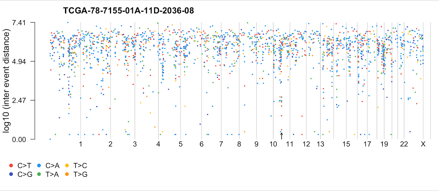
We can see from the table that the event is on chromosome 11 and consists of 7 mutations. In the plot, we see where the start of the event is as denoted by the arrow.
tcgaCompare()
36. We can compare mutation load between our samples and 33 TCGA cohorts that are built into the maftools package from the TCGA MC3 project.
First, we want to make our outer plot margins a little bigger so that our plot isn’t cut off:
par(oma=c(2,5,2,2))
Now we can run the following tcgaCompare() command to generate a plot:
tcga_luad_mutload <- tcgaCompare(maf = tcga_luad_maf, cohortName = 'Example Data', logscale = TRUE, capture_size = 35.8)
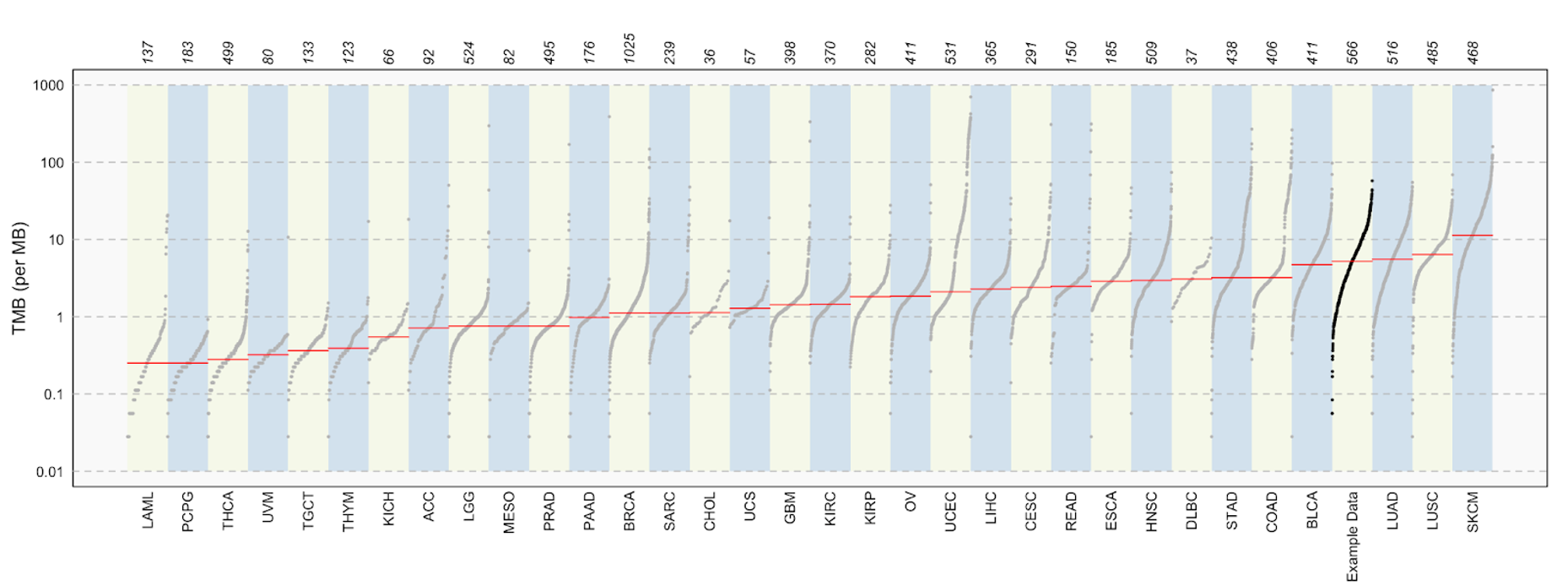
We set the capture_size parameter to 35.8 mb because this was the capture size used in the capture kit for TCGA samples.
Along the top of the plot are the case counts for each cancer type. Cancer types are along the bottom of the plot, and TMB (per MB) is on the y-axis. The red line across each cancer type is the median TMB. We can see that our group of TCGA-LUAD samples has one of the higher TMB values.
You may have noticed we are using TCGA-LUAD data, while also comparing to the LUAD cohort. The number of cases differs between these, with 566 in our dataset, and only 516 in the cohort in the maftools package. This is most likely due to a version freeze of the data included in the maftools package.
37. Before moving on, we need to reset our plot parameters, using the command:
dev.off()
somaticInteractions()
38. We can use the somaticInteractions() function to detect mutually exclusive or co-occurring sets of genes. This function performs a pair-wise Fisher’s Exact test to detect these significant interactions. This plot can be based on the top X genes in your dataset, or we can select specific genes to display.
So that the plot text and labels are not cut off in the output plot, we are going to adjust the left and top outer margins:
par(oma=c(0,1,0.5,0))
First, we will look at the top 10 genes in the TCGA-LUAD data, using the following command:
somaticInteractions(maf = tcga_luad_maf, top = 10, pvalue = c(0.05,0.1),nShiftSymbols = 2)
You will see that in addition to a plot appearing in the plot window, there is a table generated to highlight all of the mutually exclusive and co-occurrence events. This table is ordered by p-value significance.

In this plot, we can see a mutually exclusive significant interaction between KRAS and TP53, noted by the larger -log10(P-value) and the * symbol, denoting a P-value < 0.05. We can also see several significant co-occurrence interactions between TP53 and all of the other genes found in this plot.
Note: Here we have changed the nShiftSymbols parameter to 2 from a default value of 5, so that the P-value symbol legend does not overlap with the plot.
39. Now we will note the specific genes we would like to see in the plot:
somaticInteractions(maf = tcga_luad_maf, genes = c('KRAS','EGFR','ERBB4','NTRK3','NF1','PDGFRA','BRAF','ALK','ROS1','NRTK2'), pvalue = c(0.05,0.1), nShiftSymbols = 2)

In this plot, we can see a mutually exclusive significant interaction between KRAS and BRAF, KRAS and NF1, and KRAS and EGFR, noted by the larger -log10(P-value) and the * symbol, denoting a P-value < 0.05. We can also see several significant co-occurrence interactions, such as between ERBB4 and ALK.
Note: Similar to the first somaticInteractions() plot, the nShiftSymbols parameter was changed to 2 from a default value of 5, so that the P-value symbol legend does not overlap with the plot.
40. Like before, we will reset the plot parameters back to the default by using the following command:
dev.off()
41. You can use the oncoplot to double check the relationship between two genes. For example, only one sample carries both KRAS and EGFR mutations in the TCGA-LUAD cohort, validating the mutually exclusive event. This can be visualized with the following code:
oncoplot(maf = tcga_luad_maf, genes = c('KRAS','EGFR'))
OncogenicPathways() and PlotOncogenicPathways()
42. We can also use the OncogenicPathways() function to look for enrichment of known Oncogenic Signaling Pathways. This function generates a plot as well as a table (which is output to the console). Use the following command to generate both:
OncogenicPathways(maf = tcga_luad_maf)
Here is what that output table looks like:
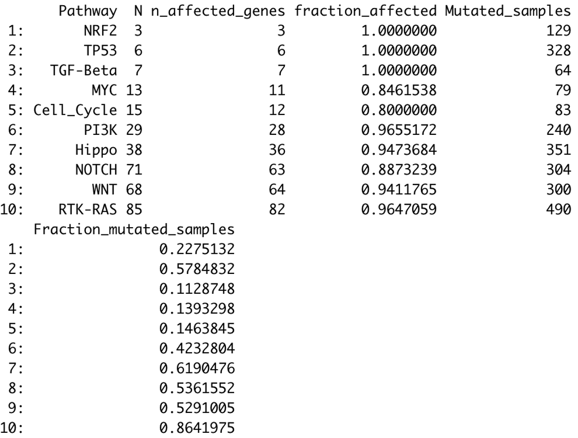
Here you see the name of the pathway (e.g., TP53 pathway), the number of genes included in the pathway, the total number of genes in the pathway affected at least in one sample, the fraction of the pathway affected, the total number of samples with mutations observed in gene of that pathway, and the overall mutational frequency of all the genes in that pathway.
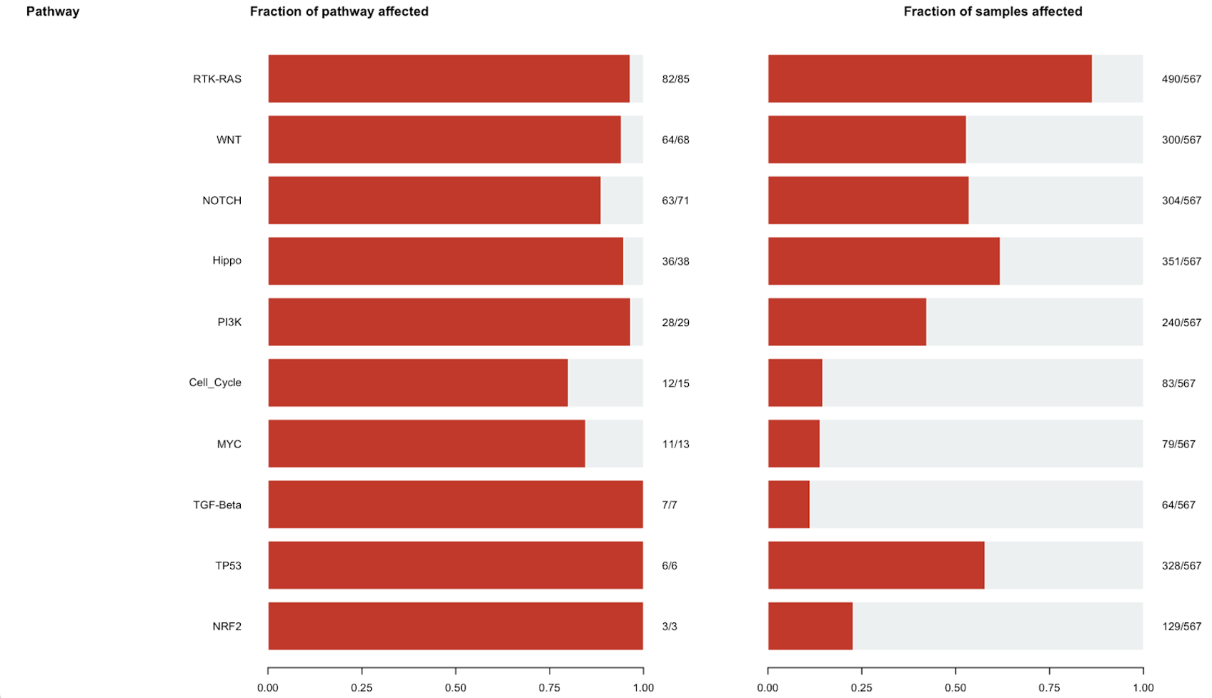
Here is a visual representation of that table in bar plot format:
43. The PlotOncogenicPathways() function allows you to visualize a pathway as an oncoplot. Use the following command to generate an oncoplot for the RTK-RAS pathway:
PlotOncogenicPathways(maf = tcga_luad_maf, pathways = "RTK-RAS")
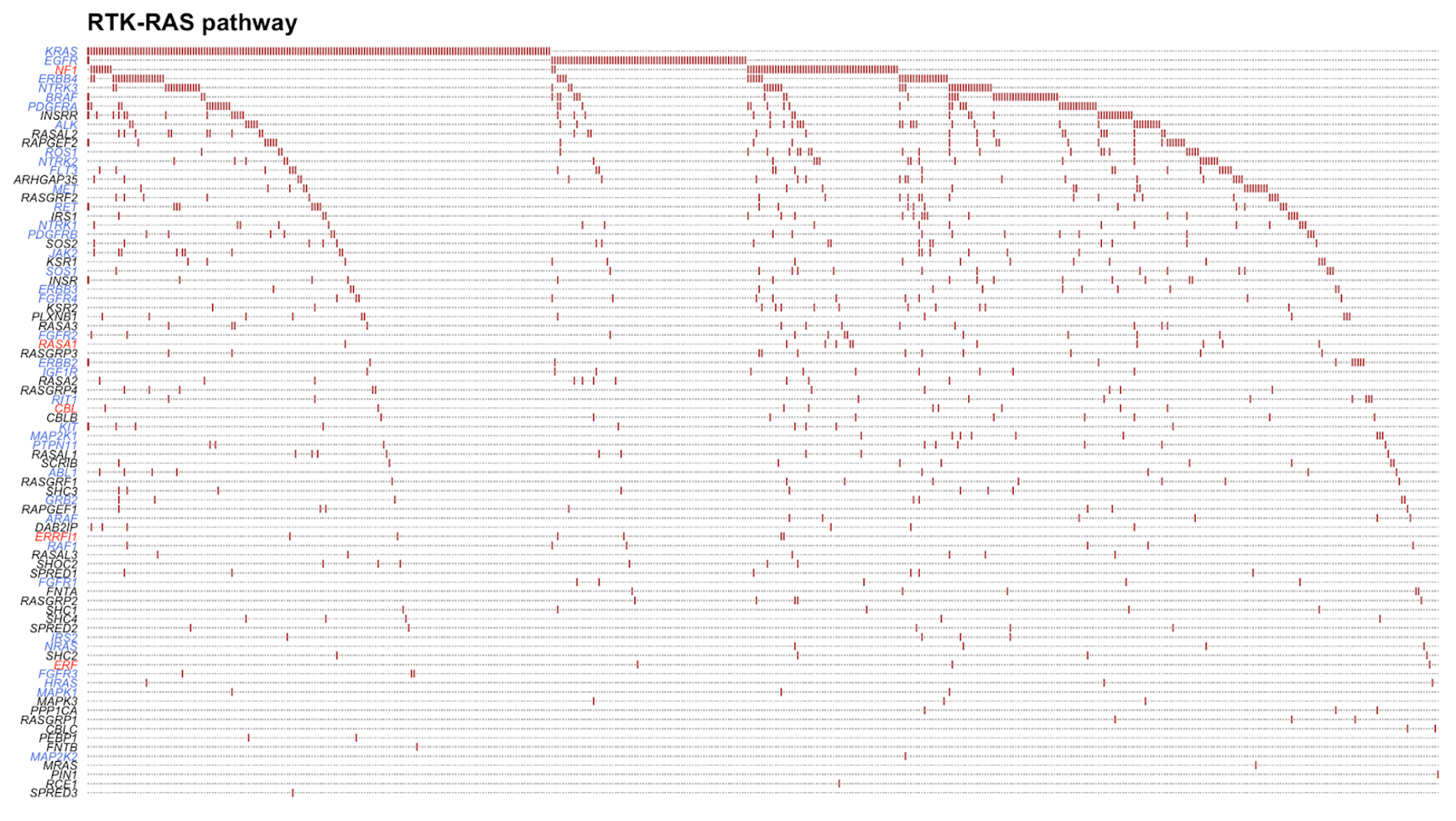
This plot visualizes the 82 genes that were mutated in almost 500 TCGA-LUAD samples. Tumor suppressor genes are colored in red and oncogenes are colored in blue. The plot orders the genes from top to bottom on the left side from most to least mutated. We can see here that KRAS is the most mutated gene in the RTK-RAS pathway, followed by EGFR and NF1.
Tip: If this appears cluttered in your Plot tab in R, click the Zoom button to open the plot in a different window.
44. We can visualize the TP53 pathway for additional practice, and to see what a less cluttered plot looks like:
PlotOncogenicPathways(maf = tcga_luad_maf, pathways = "TP53")
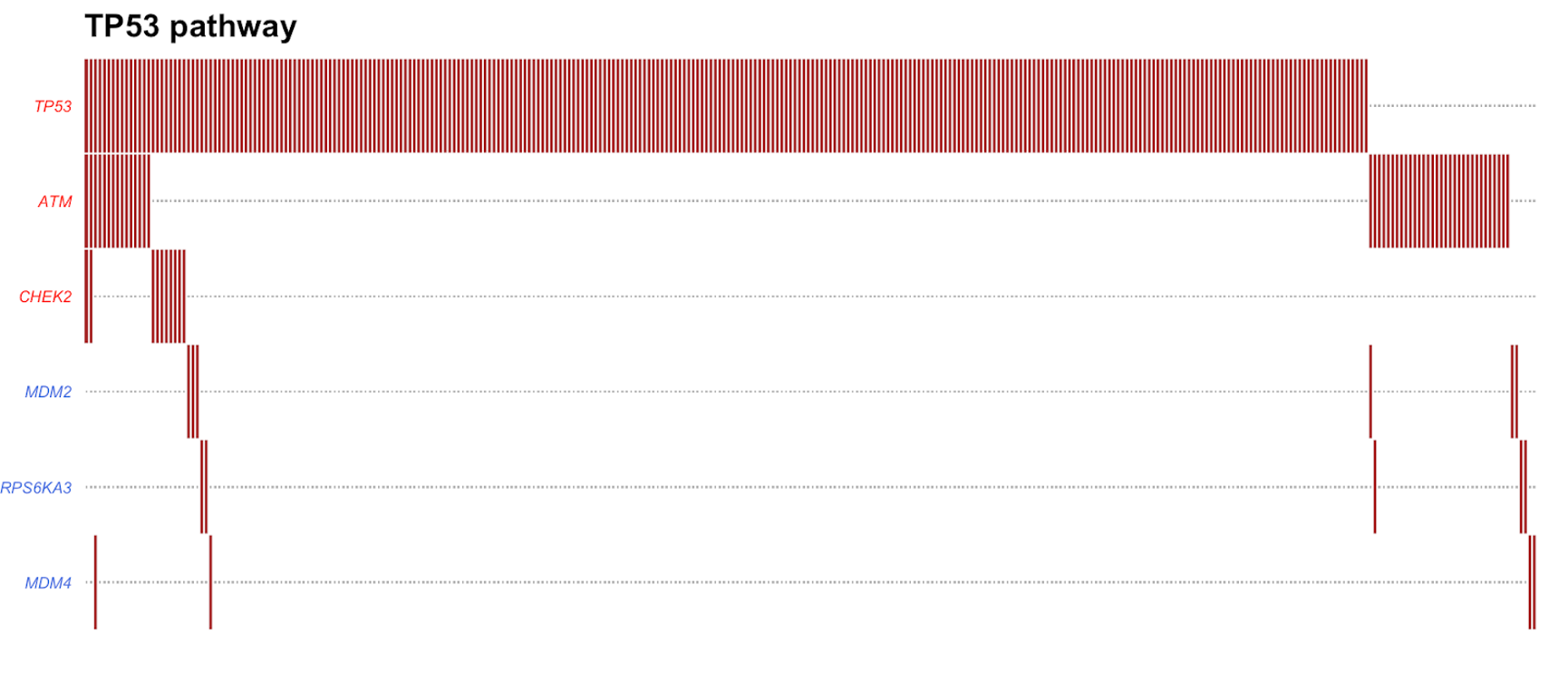
This plot visualizes the 6 genes that were mutated in over 300 TCGA-LUAD samples. Tumor suppressor genes are colored in red and oncogenes are colored in blue. The plot orders the genes from top to bottom on the left side from most to least mutated. We can see here that TP53 is the most mutated gene in the TP53 pathway, followed by ATM and CHEK2.
Tip: You can add sample names across the bottom of the plot, using the argument showTumorSampleBarcodes = TRUE. You can also include genes that are in the selected pathway but were not mutated (if applicable), using the argument fullPathway = TRUE.
45. We can save this plot to our current working directory. In the Plots window, you can select Export, and then Save as Image or Save as PDF:
Save as Image:

Save as PDF:
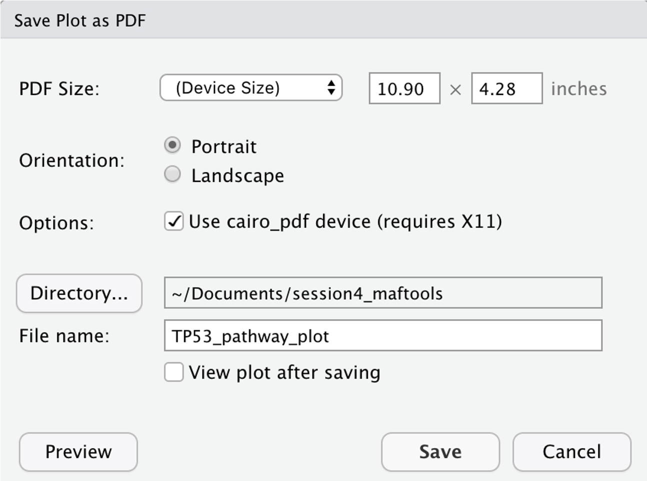
Additional Information: To save any plot automatically, before the plotting command enter pdf(file = "FILENAME.pdf") followed by dev.off(). If you do, the plot will save directly to a file instead of being displayed in RStudio. Example:
pdf(file = "FILENAME.pdf")
plotmafSummary(maf = tcga_luad_maf, rmOutlier = TRUE, addStat = 'median', dashboard = TRUE, titvRaw = FALSE)
dev.off()
Saving a plot in this way is necessary if you are running an R script in a non-interactive manner, such as a batch script on Biowulf.