Presenters: Tongwu Zhang, John McElderry
Introduction
This practical session will provide detailed steps for the SV calling by one of the most popular algorithms (e.g. Manta) from examples of analysis-ready BAM files. In addition, We will also provide example SV callings from our Sherlock-Lung study for SV filtering, annotation, and visualization. Suggestive downstream analysis related to SV will also be present in this practical session.
Preparation
Before we begin, please login to Biowulf and request an interactive session:
For a reminder on how to log-in to Biowulf, we refer you to this Biowulf HPC guide. In short:
- (Windows) use PuTTy
- (Mac) enter
ssh USERNAME@biowulf.nih.govto your terminal, then enter your password
Request an interactive session with the following command:
sinteractive --gres=lscratch:4 --mem=10g --cpus-per-task=4 --time=02:00:00
Requirements:
- Rstudio/R/R packages: tidyverse/circlize/jsonlite
To install the tidyverse, circlize, and jsonlite packages in R, you can use the install.packages() function.
# Install multiple packages at once
install.packages(c("tidyverse", "circlize", "jsonlite"))
Once the packages are installed, you can load them into your R session using the library() function
# Load the tidyverse package
library(tidyverse)

# Load the circlize package
library(circlize)

# Load the jsonlite package
library(jsonlite)
Cancer Genomics Dataset
We will use our first published Sherlock-Lung WGS data for today’s session (https://pubmed.ncbi.nlm.nih.gov/34493867/). Sherlock-Lung is a comprehensive study that aims to trace lung cancer etiology in never smokers by analyzing genomic data in tumors and surrounding lung tissue. Whole genome sequencing, whole transcriptome, genome-wide methylation, and microbiome data are being analyzed to characterize the genomic landscape of lung cancer in never smokers (LCINS) and to identify exogenous and endogenous processes involved in lung tumorigenesis.
In the first part of this practical we will analyze sliced WGS bam files from two tumor-normal pairs to identify and validate the most recurrent driver SVs, specifically focusing on the EML4-ALK fusion. In the second part, we will present the finalized SV data for visualization.
Somatic SV Calling using Illumina Manta
Manta Structural Variant Caller
Manta is a tool for the detection of structural variations (SVs) using Illumina paired-end sequencing data. It is designed to detect a wide range of SVs including insertions, deletions, inversions, and translocations. The algorithm starts by using paired-end read information to identify candidate SV breakpoints. Then, it uses split-read alignments and local assembly to further refine the breakpoint locations and genotype the SVs. Manta is highly sensitive and can detect even small SVs, it also uses paired-end and split-read evidence to genotype the events and it can handle complex SVs such as multi-allelic and large-scale events. Manta can also be used to detect somatic SVs when provided with matched normal and tumor samples.
More detailed information about the Manta algorithm can be found in the publication and GitHub page for the tool.
Understanding the function of fusion gene SVs for tumorigenesis
Since our goal is to determine the most significant fusion drivers in lung cancer among never-smokers, we would like to provide some additional background about fusion genes. Fusion genes are formed when two individual genes are joined together as a result of structural variation. Fusion genes create totally new gene products, which can result in activation of oncogenes or the inactivation of tumor suppressor genes, and then ultimately development of tumors. The specific function of a fusion gene in tumorigenesis can vary depending on the genes involved and the location of the fusion within the gene.
For example, the EML4-ALK fusion found in some cases of non-small cell lung cancer results in the activation of an oncogene, leading to the growth and spread of cancer cells. Understanding the specific function of a fusion gene can help in the development of targeted treatments for cancer. The following figure from FGviewer illustrates the impact of driver gene fusions on human cancer.

Fusion genes can participate in gene regulation in a variety of ways in cancer cells. If a partner gene, with the active promoter and dimerization functional domains, is fused with a kinase domain, it will constitutively drive the activated expression of the kinase, leading to uncontrolled cell proliferation. For example, ALK is not normally transcribed in adult lung, but under the control of the EML4 promoter, the EML4-ALK fusion gene is transcribed. The dimerization domain of EML4 permits unregulated dimerization of the tyrosine kinase domain, constitutively activating downstream pathways. The BCR-ABL1 fusion gene is formed between BCR and the non-receptor tyrosine kinase, ABL1. Lacking auto-inhibitory N-terminal myristoylation in ABL1 and dimerization function of the coiled-coil domain in BCR contribute to the constitutive activation of kinase function. TMPRSS2-ERG fusion gene has over 50% of frequency in prostate cancer patients. The strong promoter of TMPRSS2, which is a prostate tissue-specific and androgen-inducing gene, enhanced the function of proto-oncogene (ERG). Similarly, if a DNA-binding domain of FLI1 is fused with a transactivation domain of EWSR1, this fusion protein can recruit transcriptional coregulatory elements, resulting in target gene activation. Through fusion, one protein can also lose its interactions with important cellular regulators (i.e., MLL fusion genes). If the 3’-UTR region of a fusion gene is truncated during fusion, such fusion transcript can avoid the regulation by its targeting miRNAs (i.e., FGFR3-TACC3). Other FG mechanisms include the loss of function of tumor suppressors and DNA damage repairs through the deletion or frameshift open reading frame (ORF) of fusion transcripts. Recently, several studies were done for identifying downstream effectors of FGs (i.e., NUP214-ABL1, RUNX1-ETO, and SS18-SSX). SS18, which encodes the BAF complex subunit, fused with SSX and affected chromatin accessibility. - from FGViewer
It is common to observe variation in the types of fusion rearrangements and breakpoints for a given fusion pair. In the case of the EML4-ALK fusion, a large inversion structural variant (SV) is often observed between the EML4 and ALK genes on the same chromosome. Analysis and visualization of these breakpoints is crucial for understanding the consequences of this fusion.

Figure from: https://www.atcc.org/resources/application-notes/generation-of-an-eml4-alk-fusion-nsclc-isogenic-cell-line
Detailed steps for somatic SV calling using Manta
1. mkdir session6: This command creates a new directory called session6.
mkdir session6
2. cd session6: This command changes the current working directory to the newly created session6 directory.
cd session6
3. module load manta: This command loads the manta module, which is a tool for structural variant (SV) discovery.
module load manta
4. configManta.py This command runs the configManta.py script, which is used to configure the Manta workflow. The –normalBam and –tumorBam options specify the path to the normal and tumor BAM files, respectively, and the –referenceFasta option specifies the path to the reference genome in FASTA format. The –runDir option specifies the name of the directory where the Manta workflow will be run.
configManta.py \
--normalBam=/data/classes/DCEG_Somatic_Workshop/Practical_session_6/data/NSLC-0463-B01.bam \
--tumorBam=/data/classes/DCEG_Somatic_Workshop/Practical_session_6/data/NSLC-0463-T01.bam \
--referenceFasta=/data/classes/DCEG_Somatic_Workshop/Practical_session_6/reference/Homo_sapiens_assembly38.fasta \
--runDir NSLC-0463
5. runWorkflow.py: This command runs the runWorkflow.py script, which is used to execute the Manta workflow. The -m local option specifies that the workflow should be run locally, and the -j 2 option specifies that the workflow should use two CPU cores. The output of the script is redirected to the file “NSLC-0463.log” using the > operator. The 2>&1 part of the command redirects the standard error output to the same file as the standard output, so that both standard output and standard error are written to the log file.
`pwd`/NSLC-0463/runWorkflow.py -m local -j 2 >NSLC-0463.log 2>&1
6. Output the text from the log file. Use the commands less NSLC-0463.log
or more NSLC-0463.log
to see the whole log file; below we show how to preview the first 10 and last 10 lines using head and tail, respectively.
head NSLC-0463.log
[2022-12-25T02:06:43.822127] [cn4315.hpc.nih.gov] [97267_1] [WorkflowRunner] Initiating pyFlow run
[2022-12-25T02:06:43.822847] [cn4315.hpc.nih.gov] [97267_1] [WorkflowRunner] pyFlowClientWorkflowClass: MantaWorkflow
[2022-12-25T02:06:43.823592] [cn4315.hpc.nih.gov] [97267_1] [WorkflowRunner] pyFlowVersion: unknown
[2022-12-25T02:06:43.824319] [cn4315.hpc.nih.gov] [97267_1] [WorkflowRunner] pythonVersion: 2.7.15.final.0
[2022-12-25T02:06:43.825012] [cn4315.hpc.nih.gov] [97267_1] [WorkflowRunner] WorkingDir: '/spin1/users/classes/DCEG_Somatic_Workshop/Practical_session_6/session6'
[2022-12-25T02:06:43.825803] [cn4315.hpc.nih.gov] [97267_1] [WorkflowRunner] ProcessCmdLine: '/data/classes/DCEG_Somatic_Workshop/Practical_session_6/session6/NSLC-0463/runWorkflow.py -m local -j 2'
[2022-12-25T02:06:43.826535] [cn4315.hpc.nih.gov] [97267_1] [WorkflowRunner] [RunParameters] mode: local
[2022-12-25T02:06:43.827219] [cn4315.hpc.nih.gov] [97267_1] [WorkflowRunner] [RunParameters] nCores: 2
[2022-12-25T02:06:43.827873] [cn4315.hpc.nih.gov] [97267_1] [WorkflowRunner] [RunParameters] memMb: 515538
[2022-12-25T02:06:43.828533] [cn4315.hpc.nih.gov] [97267_1] [WorkflowRunner] [RunParameters] dataDir: /spin1/users/classes/DCEG_Somatic_Workshop/Practical_session_6/session6/NSLC-0463/workspace/pyflow.data
tail NSLC-0463.log
[2022-12-25T02:09:28.252005] [cn4315.hpc.nih.gov] [97267_1] [TaskManager] Completed command task: 'tabix_sortCandidateSV' launched from master workflow
[2022-12-25T02:09:28.253102] [cn4315.hpc.nih.gov] [97267_1] [TaskManager] Launching command task: 'extractSmallIndels_tabix' from master workflow
[2022-12-25T02:09:28.259460] [cn4315.hpc.nih.gov] [97267_1] [TaskRunner:extractSmallIndels_tabix] Task initiated on local node
[2022-12-25T02:09:28.369132] [cn4315.hpc.nih.gov] [97267_1] [TaskManager] Completed command task: 'extractSmallIndels_tabix' launched from master workflow
[2022-12-25T02:09:36.613797] [cn4315.hpc.nih.gov] [97267_1] [WorkflowRunner] Manta workflow successfully completed.
[2022-12-25T02:09:36.613797] [cn4315.hpc.nih.gov] [97267_1] [WorkflowRunner]
[2022-12-25T02:09:36.613797] [cn4315.hpc.nih.gov] [97267_1] [WorkflowRunner] 	workflow version: UNKNOWN
[2022-12-25T02:09:36.614994] [cn4315.hpc.nih.gov] [97267_1] [WorkflowRunner]
[2022-12-25T02:09:36.615659] [cn4315.hpc.nih.gov] [97267_1] [WorkflowRunner] Workflow successfully completed all tasks
[2022-12-25T02:09:36.616444] [cn4315.hpc.nih.gov] [97267_1] [WorkflowRunner] Elapsed time for full workflow: 172 sec
7. tree: This command runs the tree command with the -s and -h options, which show the sizes of the files and directories in “human-readable” format. The command displays the directory tree of the variants subdirectory under the results directory of the Manta workflow.
tree -sh NSLC-0463/results/variants
NSLC-0463/results/variants
├── [ 27K]  candidateSmallIndels.vcf.gz
├── [1.3K]  candidateSmallIndels.vcf.gz.tbi
├── [ 29K]  candidateSV.vcf.gz
├── [1.4K]  candidateSV.vcf.gz.tbi
├── [ 23K]  diploidSV.vcf.gz
├── [ 295]  diploidSV.vcf.gz.tbi
├── [ 22K]  somaticSV.vcf.gz
└── [ 204]  somaticSV.vcf.gz.tbi
8. module load bcftools: This command loads the “bcftools” module, which is a set of tools for manipulating variant call format (VCF) files.
module load bcftools
9. bcftools view: This command runs the bcftools view command, which is used to display the contents of a VCF file. The | operator pipes the output of the bcftools view command to the grep command, which is used to filter the output. The -v option inverts the sense of the match, so that the grep command prints only the lines that do not match the pattern “^##”.
bcftools view NSLC-0463/results/variants/somaticSV.vcf.gz |grep -v "^##"
#CHROM	POS	ID	REF	ALT	QUAL	FILTER	INFO	FORMAT	2452	NSLC-AJGA-TTP1-A-1-1-D-A79F-36
chr2	28983101	MantaDUP:TANDEM:3:0:1:0:0:0	C	<DUP:TANDEM>	.	PASS	END=28983251;SVTYPE=DUP;SVLEN=150;CIPOS=0,6;CIEND=0,6;HOMLEN=6;HOMSEQ=CTCAGC;SOMATIC;SOMATICSCORE=38	PR:SR	6,0:29,2	57,1:94,28
chr2	29225011	MantaBND:22:0:1:0:0:0:1	C	C]chr2:42299403]	.	PASS	SVTYPE=BND;MATEID=MantaBND:22:0:1:0:0:0:0;SOMATIC;SOMATICSCORE=147;BND_DEPTH=45;MATE_BND_DEPTH=66	PR:SR	34,0:76,0	57,62:83,43
chr2	42299403	MantaBND:22:0:1:0:0:0:0	C	C]chr2:29225011]	.	PASS	SVTYPE=BND;MATEID=MantaBND:22:0:1:0:0:0:1;SOMATIC;SOMATICSCORE=147;BND_DEPTH=66;MATE_BND_DEPTH=45	PR:SR	34,0:76,0	57,62:83,43
Visualization with svviz
10. module load svviz: This command loads the “svviz” module, which is a tool for visualizing structural variations.
module load svviz
11. svviz: This command runs the svviz tool with a number of options and arguments. The -t bkend option specifies the type of SV being visualized (in this case, “bkend” stands for “breakend”). The -b options specify the paths to the normal and tumor BAM files, respectively. The next three arguments specify the reference genome, the coordinates of the structural variation, and the orientation of the sequences, respectively. The –export option specifies the name of the file where the visualization should be saved, and the –annotation option specifies the path to a GTF file with gene annotations.
svviz -t bkend \
-b /data/classes/DCEG_Somatic_Workshop/Practical_session_6/data/NSLC-0463-B01.bam \
-b /data/classes/DCEG_Somatic_Workshop/Practical_session_6/data/NSLC-0463-T01.bam \
/data/classes/DCEG_Somatic_Workshop/Practical_session_6/reference/Homo_sapiens_assembly38.fasta chr2 42299403 + chr2 29225011 - \
--export NSLC-0463_EML4-ALK_fusion.svg \
--annotation /data/classes/DCEG_Somatic_Workshop/Practical_session_6/reference/genes.gtf
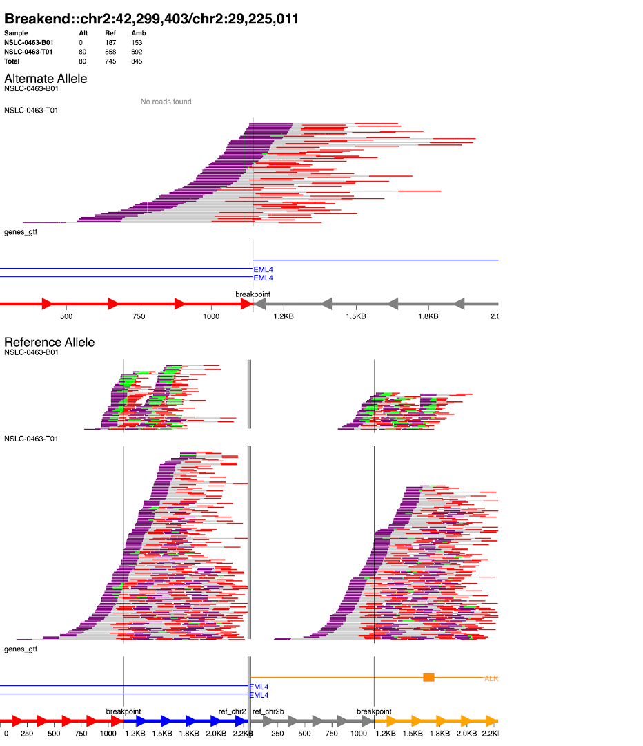
To examine the output, mount your Biowulf /data/ drive to your local computer and open the file session6/NSLC-0463_EML4-ALK_fusion.svg. (Reminder for how to do this.)
You can find more information about the svviz from the svviz official website: http://svviz.github.io/svviz/
SV Annotation
SV annotation by Illumina NIRVANA
12. Nirvana is a package developed by Illumina for variant annotation. Illumina is already installed on Biowulf and can be run on our samples easily with the following code:
module load nirvana
Run the following code:
nirvana -c $NIRVANA_DATA/Cache/GRCh38/Both \
--sd $NIRVANA_DATA/SupplementaryAnnotation/GRCh38 \
-r $NIRVANA_DATA/References/Homo_sapiens.GRCh38.Nirvana.dat \
-i NSLC-0463/results/variants/somaticSV.vcf.gz \
-o NSLC-0463
Most of these arguments are paths to databases for nirvana; to use your own variants, simply change -i to the path of your variants file and set -o to whatever filename prefix you want for your outputs. Nirvana outputs annotations in JSON format which will need to be reformatted in R or Python for better readability.
Here is the detailed information for the JSON annotation file.
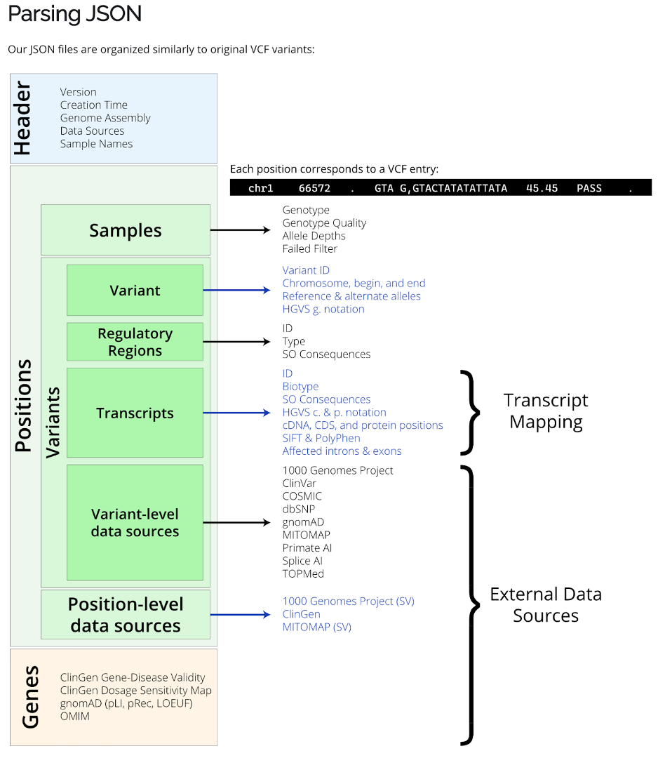
Using R studio to convert the JSON annotation file into an R data frame.
13. In R, perform the following code to extract the annotation information as a data frame, which can be easily converted to any format (e.g., txt/tsv/csv).
PLEASE NOTE: The exact data within the JSON may vary depending on the format of variants input and depending on the databases/sources used for annotating. While this code should be roughly accurate for most cases, you may need to make small changes to fit your data formatting.
library(jsonlite)
library(tidyverse)

jsondata <- fromJSON('/path/to/NSLC-0463.json.gz')

## extract the Header
jsondata %>% .[[1]] %>% as.data.frame() %>% as_tibble()

## extract the positions and all variant information
jsondata %>% .[[2]] %>% as_tibble()


## expand per-sample read support
jsondata %>% .[[2]] %>% as_tibble() %>% unnest(samples)

## expand per-sample read support, variant filtering status, and any multi-allelic sites
jsondata %>% .[[2]] %>% as_tibble() %>% unnest(samples) %>% unnest(altAlleles) %>% unnest(filters)

## extract specific variant annotations
variants_info<-jsondata %>% .[[2]] %>% as_tibble() %>% pull(variants) %>% bind_rows() %>% as_tibble()

## extract gene annotations
genes<-jsondata %>% .[[3]] %>% as_tibble()

## combine all info into one table
vars<-
  jsondata %>% .[[2]] %>%
  as_tibble() %>%
  # expand per-sample data (i.e. read support per sample)
  unnest(samples)%>%
  cbind(sample_name=jsondata[[1]]$samples)%>%
  # expand per alternate allele data
  unnest(altAlleles)%>%
  relocate(sample_name)%>%
  # join information on variants, such as population allele frequencies
  left_join(variants_info,by=c("chromosome","position"="begin","refAllele","altAlleles"="altAllele"))%>%
  select(-variants)%>%
  # expand trancript information and join gene annotations
  unnest(transcripts)%>%
  left_join(genes,by=c("hgnc"="name"))%>%
  as.tibble()

## Use this code to expand any other columns, such as clingen disease phenotypes
## if keep_empty=FALSE, variants without annotations in column clingenGeneValidity will be dropped
# vars%>%unnest(clingenGeneValidity, keep_empty=TRUE)
AnnotSV
After calling structural variants it is helpful to annotate those variants to see if any structural variants in your sample have been previously associated with disease or cancer. For this we can use the SV annotation database AnnotSV: https://www.lbgi.fr/AnnotSV/runjob.
14. Navigate to the website. For a simple example, navigate to the section that says ask for an automatic loading of this SV input file example highlighted in purple below, and in the box select yes, then hit Submit to the right.

This will submit an annotation job with their example file. In the future, you can upload your own SV files in VCF or BED format with the “Choose File” button boxed in red.
After submitting, wait ~30 seconds then refresh the page and the results should be generated like so.
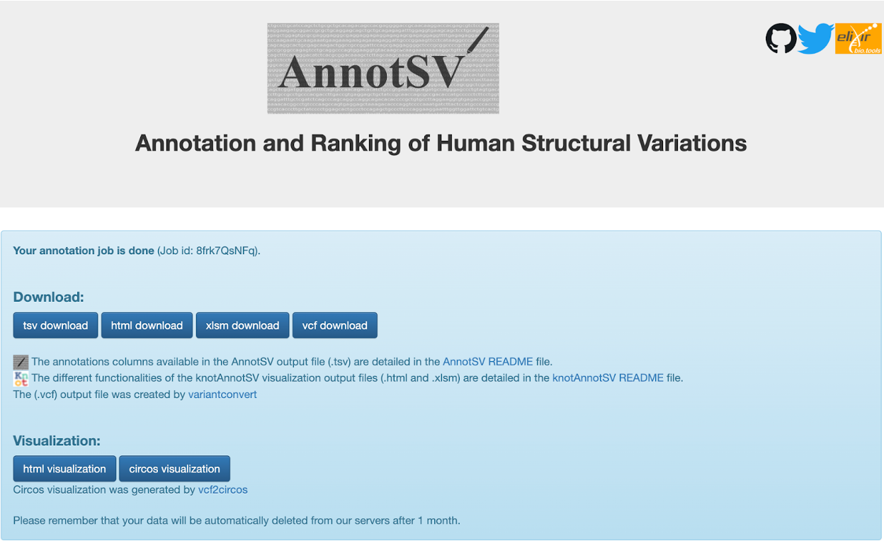
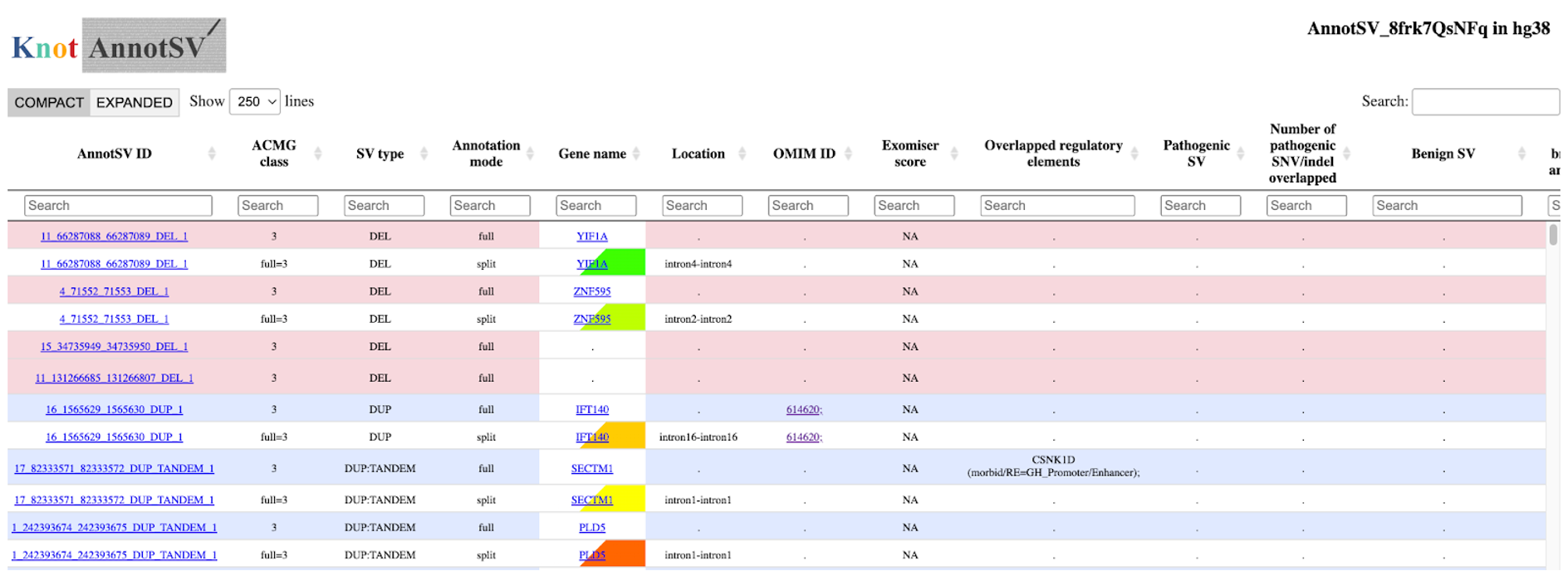
15. From here you can either download the data to your computer, or browse the output within your internet browser by clicking the bottom two buttons.
The HTML visualization will generate a colorful table in your browser with annotations such as associated genes, OMIM entries for those genes, pathogenic SVs for that gene, regulatory regions overlapping your SV, etc. Most columns you can get an explanation by hovering over the column name (full output specifications).
The circos visualization button will generate an interactive circos plot to visualize your structural variants.

(Note: you must closely match their VCF formatting specifications to generate the circos plot, otherwise AnnotSV will only generate the annotated SV table. AnnotSV asks all inputs match VCFv4.3 format.)
Fusion search and visualization with FGViewer
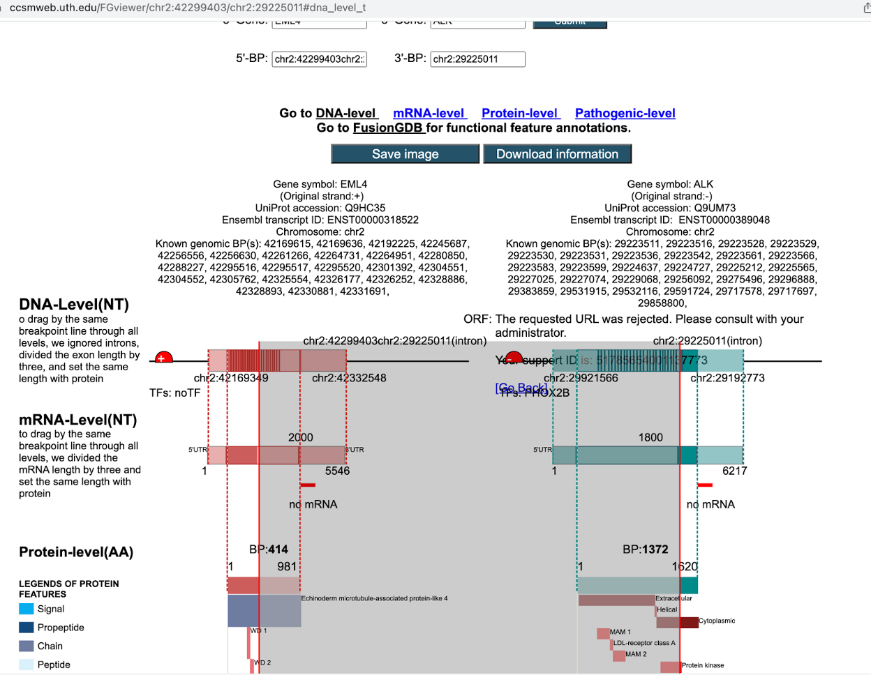
16. For the EML4-ALK fusion (translocation) from our samples, we can also check FGviewer, a tool for visualizing functional features of the human fusion gene. First, navigate to the website and click on the Search tab: https://ccsmweb.uth.edu/FGviewer.

17. Next, scroll down and in the box labelled Batch Search by Fusion Gene BPs, enter the coordinates of our EML4-ALK fusion from earlier, chr2:42299403-chr2:29225011. Then scroll to the bottom, hit the search button, and click the link labeled 0-FAM179A at the very bottom when it appears.

This will show a window where you can examine DNA-, RNA-, Protein-, and Pathogenic-level consequences of your gene fusion.
SV visualization using R
With R we have the freedom to produce graphics with greater customization. Today we will demonstrate how to use R to generate two additional figures: a barplot of the count of structural variants by type (e.g. duplication, insertion, deletion, etc.) and a circos plot to visualize where structural variants have occurred within the genome.
The following files are required for the SV visualization:
├── SV_circos.R
├── svdata.RData
└── ztw_function.R
18. You will need to download these files. Click here to download these files as a zipped folder.
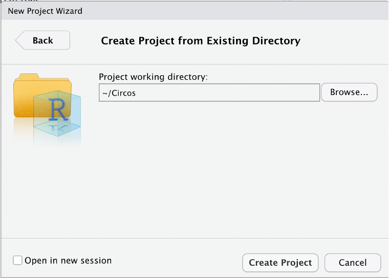
19. Now open RStudio. Go to File » New Project. A pop-up should appear to create a project; choose Existing Directory, then click Browse and select the Circos folder you just copied from Biowulf.

You should see a window like so, where the Project Working Directory ends in “/Circos”. Then hit “Create Project”.
If everything has been done properly, after R loads your window will look roughly like this with the files ztw_function.R, svdata.RData, and SV_circos.R listed in the lower-right panel.

20. In the lower right, click SV_circos.R to open the R script for our analysis in RStudio.
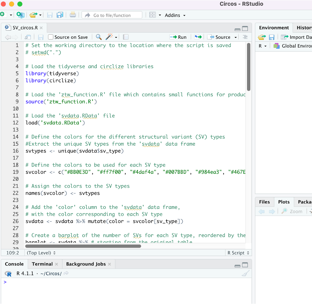
First we need to load the libraries tidyverse and circlize which contain R functions we need to run the script (lines 4-6).
# Load the tidyverse and circlize libraries
library(tidyverse)
library(circlize)
Either highlight these lines and hit Run just above the window; or copy and paste them into the console where you see the > symbol (referred to as the “prompt” and located in the bottom-left panel of RStudio by default), then hit enter.
(You may see some warning messages about the package version or R version; these warnings can be ignored. If you see an “Error”, ask for help)
21. Next, run this code in the same manner:
# Load the 'ztw_function.R' file which contains small functions for producing SV graphics
source('ztw_function.R')

# Load the 'svdata.RData' file
load('svdata.RData')
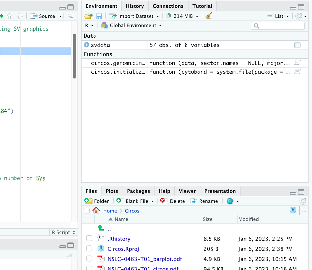
The command source runs RScripts such as ztw_function.R, which contains some helpful functions we wrote to simplify plotting. The load command will load the data from the file svdata.RData, including a table called ‘svdata’ with our SVs.
Once that code runs, in the Environment tab (top-right panel of RStudio by default) you should see the following:
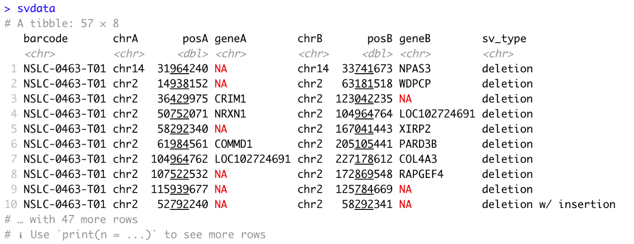
22. To preview the SV data table, within the console in the bottom-left after the prompt, >, type and enter svdata, which will yield the following:
SV Barplot
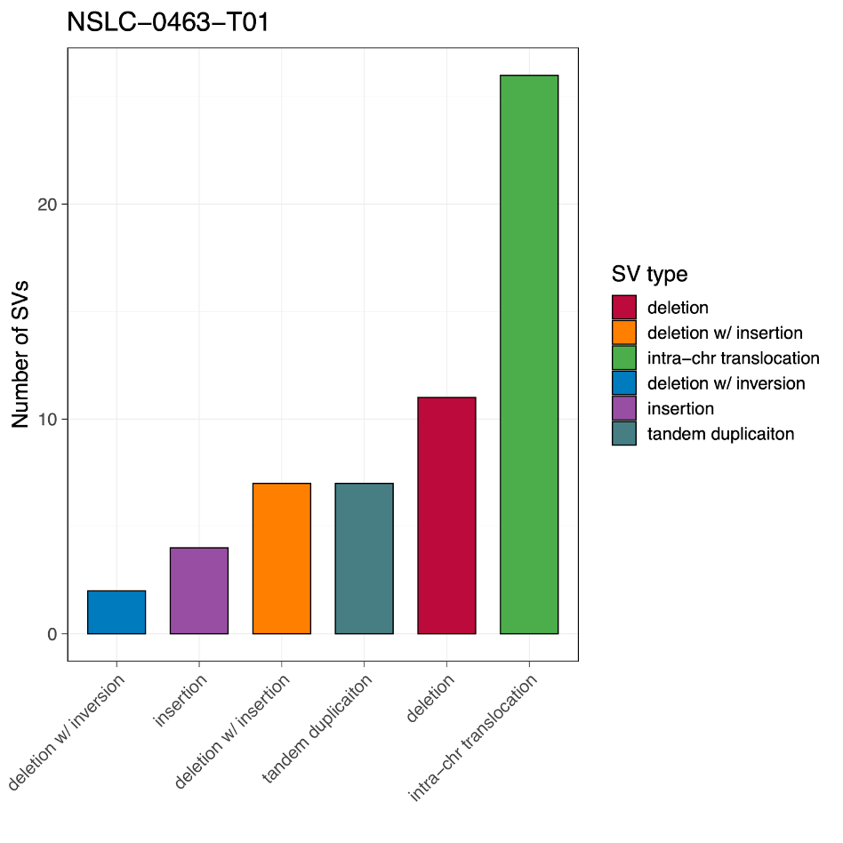
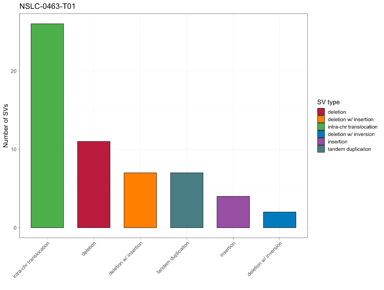
Now we have everything we need to begin plotting. Our first task is to make a barplot summarizing the number of structural variants by sv_type, like so:
23. Begin by running lines 14-26 of the script:
# Define the colors for the different structural variant (SV) types
#Extract the unique SV types from the 'svdata' data frame
svtypes <- unique(svdata$sv_type)

# Define the colors to be used for each SV type
svcolor <- c("#BB0E3D", "#ff7f00", "#4daf4a", "#007BBD", "#984ea3", "#467E84")

# Assign the colors to the SV types
names(svcolor) <- svtypes

# Add the 'color' column to the 'svdata' data frame,
# with the color corresponding to each SV type
svdata <- svdata %>% mutate(color = svcolor[sv_type])
In short, these lines of code extract the different types of SVs from our dataset for the x-axis, assign each SV type a unique color, and then add a new column color to our original SV dataset within R. Pay attention to the comments if you’re curious what each line of code does individually.
24. Once that’s run, take a look at the table once again by typing svdata into the console in the bottom left after the prompt, >. You should now see the new column which we just added called color.

25. Now finally, run the code to make the barplot, lines 28-50.
# Create a barplot of the number of SVs for each SV type, reordered by the number of SVs
barplot <- svdata %>%
  count(sv_type) %>%
  mutate(sv_type = fct_reorder(sv_type,n)) %>%
  ggplot(aes(x=sv_type,y=n,fill=sv_type)) +
  geom_col(width = 0.7, col = 'black', linewidth = 0.4) +
  scale_fill_manual(values = svcolor, breaks = names(svcolor)) +
  labs(x = '', y = 'Number of SVs', fill = 'SV type', title = 'NSLC-0463-T01') +
  theme_bw(base_size = 15, base_line_size = 0.25) +
  theme(axis.text.x = element_text(angle = 45, hjust = 1, vjust = 1))

# Show the plot
barplot
Circos Plot
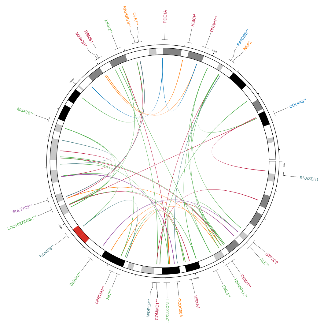
Next we will create a circos plot so we can visualize where in the genome these SVs are occurring.

26. To begin, we are going to transform our original dataset into a set of BED-formatted tables which will be easier to plot with.
- We will create the tables bed1 and bed2 which will be used to create the genomic links between SVs in the center of the circos plot
- We will also create a table bed_genes which will be used for the gene annotations along the outside of the circos
These are lines 59-107 of the script; to better understand the details read the comments:
# Adding 2000000 to the end position of the SV breakpoints when extracting the data for the Circos plot.
# By increasing the size of the breakpoints to 2 Mbp, they will be more visible in the Circos plot.
fix = 2000000

# Extract the data for the breakpoints 'A', adding 2000000 to the end position
bed1 <- svdata %>%
  mutate(posA2 = posA + fix) %>%
  select(chr = chrA, start = posA, end = posA2, color) %>%
  as.data.frame()

# Extract the data for the breakpoints 'B', adding 2000000 to the end position
bed2 <- svdata %>%
  mutate(posB2 = posB + fix) %>%
  select(chr = chrB, start = posB, end = posB2, color) %>%
  as.data.frame()

# Extract the data for the breakpoints 'A' that have associated genes, adding 2000000 to the end position
bed_gene1 <- svdata %>%
  mutate(posA2 = posA + fix) %>%
  select(chr = chrA, start = posA, end = posA2, gene = geneA, color) %>%
  filter(!is.na(gene)) %>%
  as.data.frame()

# Extract the data for the breakpoints 'B' that have associated genes, adding 2000000 to the end position
bed_gene2 <- svdata %>%
  mutate(posB2 = posB + fix) %>%
  select(chr = chrB, start = posB, end = posB2, gene = geneB, color) %>%
  filter(!is.na(gene)) %>%
  as.data.frame()

# Combine the data for the 'A' and 'B' breakpoints, group by gene, and keep only the first instance of each gene
bed_gene <- bind_rows(bed_gene1, bed_gene2) %>%
  group_by(gene) %>%
  mutate(n = length(gene)) %>%
  mutate(gene = if_else(n > 1, paste0(gene, "**"), gene)) %>%
  slice(1) %>%
  ungroup() %>%
  arrange(chr, start, end) %>%
  as.data.frame()
27. To examine any of these tables, click on its name in the Environment tab in the top right panel, or enter the name of the table at the prompt, just like we did with svdata in step 22 , and hit enter.
28. And now, finally, we will create our circos plot with the last chunk of code, lines 109 to the end of the script. We suggest running this code one section at a time to build the plot step-by-step:
28.a.
# Clear any previous plot and initialize the Circos
circos.clear()
circos.initializeWithIdeogram(plotType = NULL)
28.b.
# If there are genes associated with the SVs, add a track showing the gene locations and gene name
if(dim(bed_gene)[1]>0){
  circos.genomicLabels(bed_gene, labels.column = 4, col=bed_gene$color,side = "outside",cex = 0.4,line_lwd = 0.5,track.margin = c(0,-0.1))
} else {
  # If there are no genes associated with the SVs, add an empty track
  circos.track(ylim = c(0, 1), bg.col = NULL,bg.border="White",track.height = convert_height(6, "mm"))
}

28.c.
# initialize the Circos with chromosome labels only
circos.initializeWithIdeogram2(plotType = c("labels"))

28.d.
# initialize the Circos with chromosome axis and ideogram only
circos.initializeWithIdeogram2(plotType = c("ideogram","axis"),ideogram.height = 0.04,track.height = 0.02,major.by = 5e7 )

28.e.
# add the genomic links between two breakpoints.
if(dim(bed1)[1]>0 & dim(bed2)[1]>0 ){
  circos.genomicLink(bed1, bed2, border = NA,col = bed1$color)
}
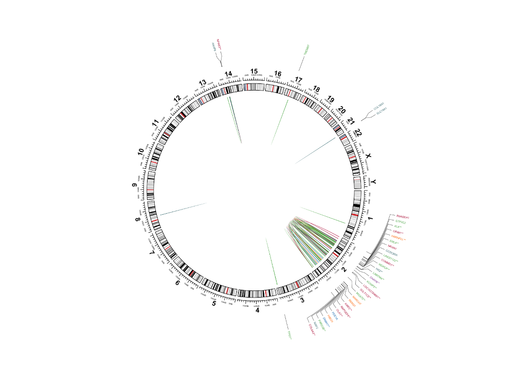
Read the comments to get an overall sense of what each code chunk does. Much of the details within each function are minor formatting operations, such as resizing, reshaping, coloring, etc.
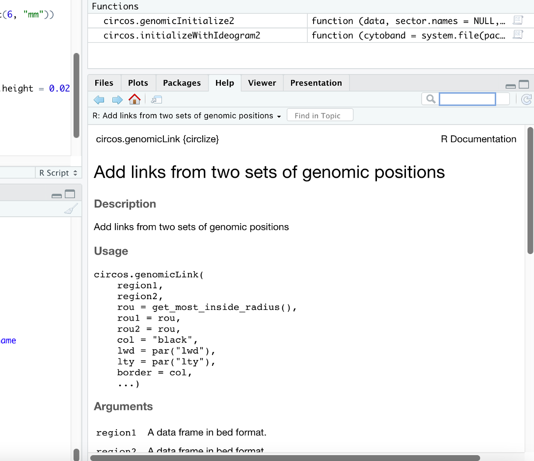
If you want to learn details about any of these plotting functions or the ones we used for the barplot, type ? followed by the name of the function, e.g. ?circos.genomicLink, and help documents for that function will appear on the lower-right panel if they are available:
OPTIONAL: Extra R practice
One of the purposes of teaching you how to use R to generate these graphs is so that you can produce graphics according to your own needs and designs. To practice doing this let’s practice modifying these two plots.
29. Let’s return to the barplot we generated. Here we suggest two challenge exercises; in order of difficulty:
a. Reverse the order of the bars, from most to least
b. Change the x-axis to be samples instead of SV type so that the SV types are stacked in a single bar (this could be useful for instance if you were visualizing several samples at once)
See the images below for examples:

To accomplish part a, first think about what section of the code handles sorting our SV table entries. Does this command have any built-in options to accomplish what we want? Are there any other ways to accomplish this?
Answer for part a
The command that sorts our samples is this one on line 31:
mutate(sv_type = fct_reorder(sv_type,n)) %>%Specifically, the command fct_reorder is really what’s doing the work to sort and it’s what we need to change. If you enter
?fct_reorderand read the help documents you’ll see that fct_reorder has an option .desc; if we set that option to TRUE then we’ll get the desired result.mutate(sv_type = fct_reorder(sv_type,n,.desc=TRUE)) %>%Alternatively, the function sorts in increasing order by default. Thus, if we sort by the negative of count ‘n’ we’ll reverse the sorting order.
mutate(sv_type = fct_reorder(sv_type,-n)) %>%
For b, we need to change the section of code that defines the x-axis of the plot from SV types to samples. How can we accomplish this?
Answer for part b
The part of our plotting code that handles the axes is this one on line 32:
ggplot(aes(x=sv_type,y=n,fill=sv_type)) +If we quickly review our starting table we can see that the column storing our sample information is called ‘barcode’:
> svdata
# A tibble: 57 × 9
   barcode       chrA       posA geneA        chrB       posB geneB        sv_type             color
   <chr>         <chr>     <dbl> <chr>        <chr>     <dbl> <chr>        <chr>               <chr>
 1 NSLC-0463-T01 chr14  31964240 NA           chr14  33741673 NPAS3        deletion            #BB0…
 2 NSLC-0463-T01 chr2   14938152 NA           chr2   63181518 WDPCP        deletion            #BB0…
 3 NSLC-0463-T01 chr2   36429975 CRIM1        chr2  123042235 NA           deletion            #BB0…
 4 NSLC-0463-T01 chr2   50752071 NRXN1        chr2  104964764 LOC102724691 deletion            #BB0…
 5 NSLC-0463-T01 chr2   58292340 NA           chr2  167041443 XIRP2        deletion            #BB0…
 6 NSLC-0463-T01 chr2   61984561 COMMD1       chr2  205105441 PARD3B       deletion            #BB0…
 7 NSLC-0463-T01 chr2  104964762 LOC102724691 chr2  227178612 COL4A3       deletion            #BB0…
 8 NSLC-0463-T01 chr2  107522532 NA           chr2  172869548 RAPGEF4      deletion            #BB0…
 9 NSLC-0463-T01 chr2  115939677 NA           chr2  125784669 NA           deletion            #BB0…
10 NSLC-0463-T01 chr2   52792240 NA           chr2   58292341 NA           deletion w/ insert… #ff7…
# … with 47 more rows
# ℹ Use `print(n = ...)` to see more rows
So if we change “x=” from sv_type to barcode like so, we’ll have our graph setup:
ggplot(aes(x=barcode,y=n,fill=sv_type)) +. If you try to run this code you’ll encounter an error however:
> barplot
Error in `geom_col()`:
! Problem while computing aesthetics.
ℹ Error occurred in the 1st layer.
Caused by error in `FUN()`:
! object 'barcode' not found
Run `rlang::last_error()` to see where the error occurred.
To see why, run just this code to see what our data table looks like after these commands, and just before we go to generate our barplot:
svdata %>%
  count(sv_type) %>%
  mutate(sv_type = fct_reorder(sv_type,n))
barcode isn’t in our table anymore; the only columns are sv_type and n because the count() command reduces the original table only down to the variables being counted and their count totals in column n. To fix this we can simply count by both sample and sv_type, like so:
count(barcode,sv_type) %>%If you make both of these changes you’ll get the following code and the stacked barplot above:
svdata %>%
  count(barcode,sv_type) %>%
  mutate(sv_type = fct_reorder(sv_type,n)) %>%
  ggplot(aes(x=barcode,y=n,fill=sv_type)) +
  geom_col(width = 0.7, col = 'black', linewidth = 0.4) +
  scale_fill_manual(values = svcolor, breaks = names(svcolor)) +
  labs(x = '', y = 'Number of SVs', fill = 'SV type', title = 'NSLC-0463-T01') +
  theme_bw(base_size = 15, base_line_size = 0.25) +
  theme(axis.text.x = element_text(angle = 45, hjust = 1, vjust = 1))
30. Next let’s try to customize the circos plot. In the original figure we observed many structural variants on chromosome 2, so let’s try producing a circos plot where we zoom in only on chromosome 2, like so:
To do this we need to accomplish a couple of things:
- Limit our structural variants table to only chr2, and reduce the extra bp padding added to the end positions since this graph is much smaller
- Limit the ideogram to only chr2
The first task requires filtering the tables bed1, bed2, and bed_genes to just the SVs/genes on chr2. We can accomplish this by adding a filter command somewhere in the code for making these three tables. Get the help documents for this command with ?filter and see if you can get generate these tables. If you get stuck, check the answer in the dropdown below.
How to generate new tables
# Extract the data for the breakpoints 'A', adding 200000 to the end position
bed1_chr2 <- svdata %>%
  filter(chrA=="chr2",chrB=="chr2")%>% ## filter to variants starting and ending in chr2
  mutate(posA2 = posA + 200000) %>%
  select(chr = chrA, start = posA, end = posA2, color) %>%
  as.data.frame()

# Extract the data for the breakpoints 'B', adding 200000 to the end position
bed2_chr2 <- svdata %>%
  filter(chrA=="chr2",chrB=="chr2")%>% ## filter to variants starting and ending in chr2
  mutate(posB2 = posB + 200000) %>%
  select(chr = chrB, start = posB, end = posB2, color) %>%
  as.data.frame()

# Filter the gene annotation track
bed_gene_chr2<-bed_gene%>%filter(chr=="chr2")
Once we have the tables, we need to limit the ideogram to only chr2 and plot using the tables we just generated in the first part. To change the ideogram, think about which parts of the circos code handled the various parts of the ideogram (Hint: these parts of the code are very appropriately named).
We should also do some re-styling to get it looking right. Try this exercise yourself, and use the answer below if you get stuck.
Answer for reformatting the circos
To every circos.initializeWithIdeogram and circos.initializeWithIdeogram2 command we need to add the variable chromosome.index=”chr2” which filters to a subset of chromosomes. Then swap every mention of bed1, bed2, and bed_gene for the new tables generated in the first part. This will be the finished code chunk:
# Clear any previous plot and initialize the Circos
circos.clear()
circos.initializeWithIdeogram(plotType = NULL,chromosome.index = "chr2")

# If there are genes associated with the SVs, add a track showing the gene locations and gene name
if(dim(bed_gene)[1]>0){
  circos.genomicLabels(bed_gene%>%filter(chr=="chr2"), labels.column = 4, col=bed_gene$color,side = "outside",cex = 0.4,line_lwd = 0.5,track.margin = c(0,-0.1))
} else {
  # If there are no genes associated with the SVs, add an empty track
  circos.track(ylim = c(0, 1), bg.col = NULL,bg.border="White",track.height = convert_height(6, "mm"))
}

# initialize the Circos with chromosome labels only
circos.initializeWithIdeogram2(plotType = c("labels"))
# initialize the Circos with chromosome axis and ideogram only
circos.initializeWithIdeogram2(plotType = c("ideogram","axis"),ideogram.height = 0.04,track.height = 0.02,major.by = 5e7,chromosome.index = "chr2")

# add the genomic links between two breakpoints.
if(dim(bed1)[1]>0 & dim(bed2)[1]>0 ){
  circos.genomicLink(bed1_chr2, bed2_chr2, border = NA,col = bed1_chr2$color)
}
When you generate this plot it will look close to what we want, but not perfect. Specifically, the genes are rather far from the axes, and the gene names are a little small.
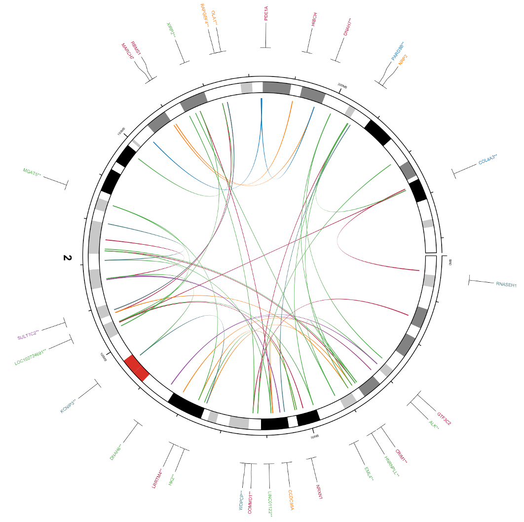
To fix this, we can remove the chromosome label since there’s only one chromosome (or if you like the label set the chr label’s track.height variable to a very small number), then increase the variable cex in the command for circos.genomicLabels. Here’s the final code:
# Clear any previous plot and initialize the Circos
circos.clear()
circos.initializeWithIdeogram(plotType = NULL,chromosome.index = "chr2")

# If there are genes associated with the SVs, add a track showing the gene locations and gene name
if(dim(bed_gene)[1]>0){
  circos.genomicLabels(bed_gene%>%filter(chr=="chr2"), labels.column = 4, col=bed_gene$color,side = "outside",cex = 0.6,line_lwd = 0.5,track.margin = c(0,-0.1))
} else {
  # If there are no genes associated with the SVs, add an empty track
  circos.track(ylim = c(0, 1), bg.col = NULL,bg.border="White",track.height = convert_height(6, "mm"))
}

# initialize the Circos with chromosome labels only
# circos.initializeWithIdeogram2(plotType = c("labels"),track.height = 0.0000001)
# initialize the Circos with chromosome axis and ideogram only
circos.initializeWithIdeogram2(plotType = c("ideogram","axis"),ideogram.height = 0.04,track.height = 0.02,major.by = 5e7,chromosome.index = "chr2")

# add the genomic links between two breakpoints.
if(dim(bed1)[1]>0 & dim(bed2)[1]>0 ){
  circos.genomicLink(bed1_chr2, bed2_chr2, border = NA,col = bed1_chr2$color)
}
Advanced genomic analysis based on SV callings
SV signature analysis
Structural variant (SV) signature analysis is a method used to identify and characterize the specific patterns of SVs in a genome. This can include identifying the specific genes or regions that are most frequently affected by SVs, as well as the types of SVs that are present (such as deletions, duplications, inversions, or translocations). By analyzing the SV signatures in a genome, researchers can gain insight into the underlying mechanisms that drive the development of genomic rearrangements and the role they play in disease. For example, Li et al., published a SV signature analysis in nature 2020 (link). They developed methods to group, classify and describe somatic structural variants, using data from the Pan-Cancer Analysis of Whole Genomes (PCAWG) Consortium of the International Cancer Genome Consortium (ICGC) and The Cancer Genome Atlas (TCGA), which aggregated whole-genome sequencing data from 2,658 cancers across 38 tumour types. From that study, they detected sixteen signatures of structural variations. This study shows that a wide variety of rearrangement processes are active in cancer, which generate complex configurations of the genome upon which selection can act.
Identification of complex genomic rearrangements
Complex genomic rearrangements refer to large-scale changes in the genome that involve multiple structural variants (SVs) occurring in close proximity. One example of this is Chromothripsis, which is a phenomenon where multiple, clustered SVs occur within a single chromosome in a single event, leading to significant genomic changes. Identification of these complex genomic rearrangements can provide important insight into the underlying mechanisms of disease and the role that genomic instability plays in the development of cancer and other genetic disorders. As part of the Pan-Cancer Analysis of Whole Genomes (PCAWG) Consortium of the International Cancer Genome Consortium (ICGC) and The Cancer Genome Atlas (TCGA), Researchers analyze patterns of chromothripsis across 2,658 tumors from 38 cancer types using whole-genome sequencing data (link). They find that chromothripsis events are pervasive across cancers, with a frequency of more than 50% in several cancer types. You can find more information about chromothripsis including the detecting algorithm, and patterns across all cancer types in Chromothripsis Explorer.
Integrative analysis with other genomic or clinical data
Integrative analysis refers to the combination of different types of data to gain a more comprehensive understanding of a biological system. This can include combining SV signature analysis with other genomic data, such as gene expression or epigenetic data, as well as clinical data, such as patient outcomes or treatment response. By integrating these different types of data, researchers can gain a more complete understanding of the underlying mechanisms of disease and the role that SVs play in the development of cancer and other genetic disorders.